
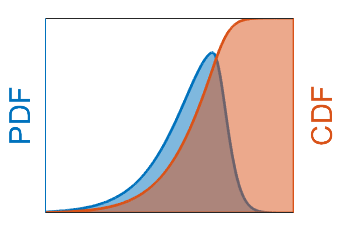
Generalized chi-square distribution 
gx2 is a python package that computes the statistics, characteristic function, pdf, cdf, inverse cdf,
random numbers, and exact gradients/Hessians of the cdf, of the generalized chi-square distribution.
This is the python port of the
MATLAB toolbox.
A generalized chi-square variable is a weighted sum of independent non-central chi-square variables plus a normal variable — equivalently, the quadratic form of a normal random vector. It is parametrized by:
| parameter | meaning |
|---|---|
w |
weights of the non-central chi-square terms |
k |
their degrees of freedom |
l |
their non-centralities |
s |
scale (standard deviation) of the added normal term |
m |
constant offset |
Author and citation
Abhranil Das, Center for Perceptual Systems, The University of Texas at Austin. Bugs / comments / questions / suggestions to abhranil.das@utexas.edu.
If you use this code, please cite:
- A method to integrate and classify normal distributions
- New methods to compute the generalized chi-square distribution
Installation
pip install gx2
Requires numpy, scipy and mpmath. matplotlib is optional, for plotting
in the getting-started notebook.
Public functions
| function | purpose |
|---|---|
gx2_to_norm_quad_params(w, k, l, s, m) |
native gx2 parameters → quadratic-form parameters of a standard normal |
norm_quad_to_gx2_params(mu, v, quad, merge=) |
normal and quadratic-form parameters → native gx2 parameters |
stat(w, k, l, s, m) |
mean, variance, and mode of a gx2 distribution |
rnd(w, k, l, s, m, size=, method=) |
random numbers |
char(t, w, k, l, s, m) |
characteristic function |
cdf(x, w, k, l, s, m, side=, method=, ...) |
cdf |
pdf(x, w, k, l, s, m, side=, method=, ...) |
|
inv(p, w, k, l, s, m, side=, method=, ...) |
inverse cdf |
norm_err(mu0, v0, mu1, v1, quad, p0=, p1=, grad=, hess=, ...) |
classification error between two normal classes separated by the optimal quadratic boundary, and optionally its gradient/Hessian wrt the boundary coefficients q2, q1, q0 |
cdf_grad_gx2(x, w, k, l, s, m, wrt=, hess=, ...) |
exact (not finite-differenced) gradient and Hessian of the cdf wrt the native parameters w, k, l, s, m |
cdf_grad_norm_quad(x, mu, v, quad, wrt=, hess=, ...) |
exact gradient and Hessian of the cdf wrt the quadratic boundary coefficients q2, q1, q0 |
opt_norm_quad_bd(mu0, v0, mu1, v1, p0=, p1=) |
optimal (Bayes) quadratic boundary between two normal classes, for use with norm_err/cdf_grad_norm_quad |
For full documentation of any function, use Python's help (or ? in
Jupyter), e.g.:
help(gx2.gx2_to_norm_quad_params)
help(gx2.norm_quad_to_gx2_params)
help(gx2.stat)
help(gx2.rnd)
help(gx2.char)
help(gx2.cdf)
help(gx2.pdf)
help(gx2.inv)
help(gx2.norm_err)
help(gx2.cdf_grad_gx2)
help(gx2.cdf_grad_norm_quad)
help(gx2.opt_norm_quad_bd)
Computation methods for cdf / pdf
method='auto' (default) picks a good method for the given parameters. You can
also force one:
| method | notes |
|---|---|
'imhof' |
Imhof–Davies numerical integration (precision='basic' or 'vpa') |
'ray' |
ray-trace method (precision='basic', 'log' or 'vpa'; tune with n_rays, force_mc) |
'ifft' |
inverse-FFT method; x='full' returns the cdf/pdf over a spanning grid |
'ruben' |
Ruben's series — requires all w the same sign and s=0 |
'tail' |
infinite-tail approximation |
'pearson' |
Pearson's 3-moment approximation |
'ellipse' |
ellipse approximation near a finite tail — requires all w the same sign and s=0 |
Examples
The following are the worked examples of the interactive GettingStarted.ipynb notebook.
import warnings
import numpy as np
import matplotlib.pyplot as plt
import gx2

# Keep this getting-started's output clean. The far-tail sections below
# deliberately push the methods past the limits of double precision, which
# would otherwise print expected underflow / log10-of-zero warnings.
warnings.filterwarnings("ignore")
np.seterr(all="ignore")

np.random.seed(0)  # for reproducible random samples below
Calculate mean, variance, mode
# gx2 parameters
w = [1, -10, 2]
k = [1, 2, 3]
l = [2, 3, 7]
s = 5
m = 10

mu, v, mode = gx2.stat(w, k, l, s, m, mode=True)
print("mu   =", mu)
print("v    =", v)
print("mode =", mode)
mu   = -17.0
v    = 1771.0
mode = 9.297513876130134
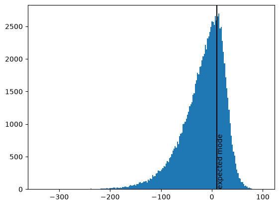
Generate random samples
r = gx2.rnd(w, k, l, s, m, size=(1, int(1e5)))
plt.figure()
plt.hist(r.ravel(), bins=200, edgecolor='none')
plt.axvline(mode, color='k')
plt.text(mode, 0, 'expected mode', rotation=90, va='bottom')
plt.show()
Compute PDF, CDF and inverse CDF with default methods
x = [10, 25]
f = gx2.pdf(x, w, k, l, s, m)
print("f =", f)
p = gx2.cdf(x, w, k, l, s, m)
print("p =", p)
# find the median by using the inverse CDF function:
x_med = gx2.inv(.5, w, k, l, s, m)
print("x_med =", x_med)
# Compute quantiles for cdf values of 1e-3 and 1e-2, by supplying their log10 values:
x_q = gx2.inv([-3, -2], w, k, l, s, m)
print("x_q =", x_q)
# verify that cdf values here are indeed 1e-3 and 1e-2
print("p =", gx2.cdf(x_q, w, k, l, s, m))
# Compute quantiles for complementary cdf values of 1e-3 and 1e-2, by supplying their log10 values:
x_q = gx2.inv([-3, -2], w, k, l, s, m, side='upper')
print("x_q (upper) =", x_q)
# verify that ccdf values here are indeed 1e-3 and 1e-2
print("p (upper) =", gx2.cdf(x_q, w, k, l, s, m, side='upper'))
f = [0.01205709 0.00879803]
p = [0.71497983 0.87899866]
x_med = -8.765662415017411
x_q = [-218.36937302 -149.26056464]
p = [0.001 0.01 ]
x_q (upper) = [69.48993111 51.03378046]
p (upper) = [0.001 0.01 ]
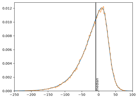
# compute the PDF over most of the span of the distribution.
# with the 'full' argument, the span x is computed automatically.
f, _, xf = gx2.pdf('full', w, k, l, s, m)

# now compare the sampled histogram with the computed PDF
plt.figure()
plt.plot(xf, f)
plt.hist(r.ravel(), bins=200, density=True, histtype='step')
plt.axvline(x_med, color='k')  # mark the computed median
plt.text(x_med, 0, 'median', rotation=90, va='bottom')
plt.xlim([-250, 100])
plt.show()
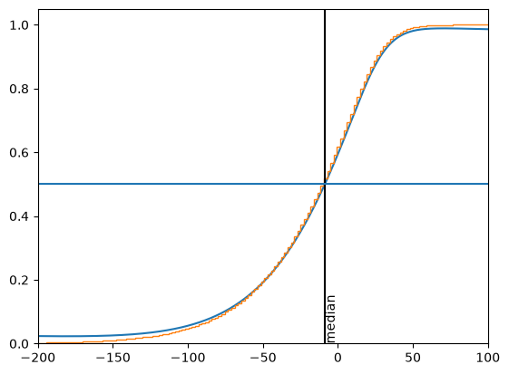
# compute CDF over most of the span of the distribution.
# the 'full' argument uses the IFFT method, good for quick rough plots,
# but less accurate (esp. for CDF) than some other methods
p, _, xp = gx2.cdf('full', w, k, l, s, m)

# now compare the sampled histogram with the computed CDF
plt.figure()
plt.plot(xp, p)
plt.hist(r.ravel(), bins=200, density=True, cumulative=True, histtype='step')
# mark the computed median, and verify that it sits at 0.5 on the vertical axis:
plt.axvline(x_med, color='k')
plt.text(x_med, 0, 'median', rotation=90, va='bottom')
plt.axhline(0.5)
plt.xlim([-200, 100])
plt.show()
Compute CDF, PDF and inverse CDF with each exact method and its settings
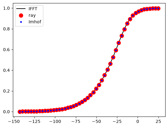
A non-elliptic distribution
w = [-2, -5, 2]
k = [2, 1, 3]
l = [0, 4, 4]
s = 3
m = -20

# first find the quantile points at 0.1% in each tail
x_bounds = gx2.inv([0.001, 0.999], w, k, l, s, m)
print("x_bounds =", x_bounds)
# now compute within this range
x = np.linspace(x_bounds[0], x_bounds[1], 50)

# compute CDF
p_ifft = gx2.cdf(x, w, k, l, s, m, method='ifft')
p_imhof = gx2.cdf(x, w, k, l, s, m, method='imhof')
p_ray = gx2.cdf(x, w, k, l, s, m, method='ray', n_rays=int(1e4))

# plot markers largest first, smallest last, so overlapping dots all stay visible
plt.figure()
plt.plot(x, p_ifft, '-k', label='IFFT')
plt.plot(x, p_ray, 'or', markersize=9, label='ray')
plt.plot(x, p_imhof, '.b', markersize=6, label='Imhof')
plt.legend()
plt.show()
# compute PDF
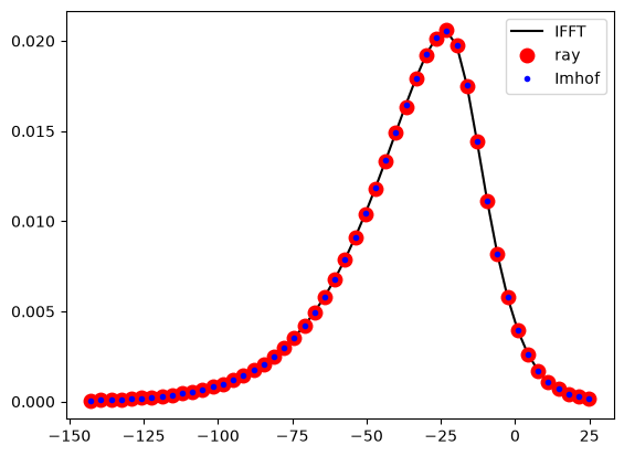
f_ifft = gx2.pdf(x, w, k, l, s, m, method='ifft')
f_imhof = gx2.pdf(x, w, k, l, s, m, method='imhof')
f_ray = gx2.pdf(x, w, k, l, s, m, method='ray', n_rays=int(1e6))

# plot markers largest first, smallest last, so overlapping dots all stay visible
plt.figure()
plt.plot(x, f_ifft, '-k', label='IFFT')
plt.plot(x, f_ray, 'or', markersize=9, label='ray')
plt.plot(x, f_imhof, '.b', markersize=6, label='Imhof')
plt.legend()
plt.show()
# Compute quantiles for tiny cdf values of 1e-1000 and 1e-2000, by supplying
# their log10 values. Use a forward cdf method that can get down to such tiny values.
# Here we use the infinite-tail approximation.
x_q = gx2.inv([-1e3, -2e3], w, k, l, s, m, method='tail')
print("x_q =", x_q)
# now verify using an exact cdf method that cdf values here are indeed 1e-1000 and 1e-2000:
print("p =", gx2.cdf(x_q, w, k, l, s, m, method='ray', n_rays=int(1e7)))
# now do the same for the upper tail:
x_q = gx2.inv([-1e3, -2e3], w, k, l, s, m, side='upper', method='tail')
print("x_q (upper) =", x_q)
print("p (upper) =", gx2.cdf(x_q, w, k, l, s, m, side='upper', method='ray', n_rays=int(1e7)))
x_q = [-24365.14269438 -47950.03867407]
p = [-1006.24736289 -2014.43928422]
x_q (upper) = [ 9723.84451406 19159.3719629 ]
p (upper) = [ -999.44410366 -2000.06198604]
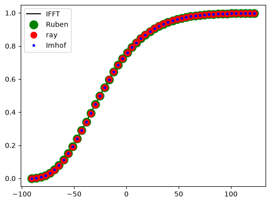
An elliptic distribution
Here we can use Ruben's method too.
w = [3, 4, 5]
k = [1, 2, 3]
l = [2, 3, 7]
s = 0
m = -100

# first find the quantile points at 0.1% in each tail
x_bounds = gx2.inv([0.001, 0.999], w, k, l, s, m)
print("x_bounds =", x_bounds)
# now compute within this range
x = np.linspace(x_bounds[0], x_bounds[1], 50)

# compute CDF
p_ifft = gx2.cdf(x, w, k, l, s, m, method='ifft')
p_imhof = gx2.cdf(x, w, k, l, s, m, method='imhof')
p_ray = gx2.cdf(x, w, k, l, s, m, method='ray', n_rays=int(1e4))
p_ruben = gx2.cdf(x, w, k, l, s, m, method='ruben')

# plot markers largest first, smallest last, so overlapping dots all stay visible
plt.figure()
plt.plot(x, p_ifft, '-k', label='IFFT')
plt.plot(x, p_ruben, 'og', markersize=12, label='Ruben')
plt.plot(x, p_ray, 'or', markersize=9, label='ray')
plt.plot(x, p_imhof, '.b', markersize=6, label='Imhof')
plt.legend()
plt.show()
# compute PDF
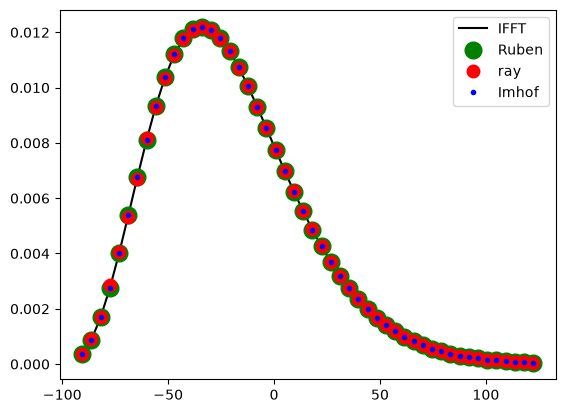
f_ifft = gx2.pdf(x, w, k, l, s, m, method='ifft')
f_imhof = gx2.pdf(x, w, k, l, s, m, method='imhof')
f_ray = gx2.pdf(x, w, k, l, s, m, method='ray', n_rays=int(1e6))
f_ruben = gx2.pdf(x, w, k, l, s, m, method='ruben')

# plot markers largest first, smallest last, so overlapping dots all stay visible
plt.figure()
plt.plot(x, f_ifft, '-k', label='IFFT')
plt.plot(x, f_ruben, 'og', markersize=12, label='Ruben')
plt.plot(x, f_ray, 'or', markersize=9, label='ray')
plt.plot(x, f_imhof, '.b', markersize=6, label='Imhof')
plt.legend()
plt.show()
# Compute quantiles for tiny cdf values of 1e-1000 and 1e-2000, by supplying
# their log10 values. Use a forward cdf method that can get down to such tiny values.
# Here we use the ellipse approximation, with x_scale='log', which allows to specify
# log10 values of x measured from the finite tail m.
x_q = gx2.inv([-1e3, -2e3], w, k, l, s, m, method='ellipse', x_scale='log')
print("x_q =", x_q)
# this means that the computed quantiles are 1e-331 and 1e-664 above m

# now verify using the forward cdf method that cdf values here are indeed 1e-1000 and 1e-2000:
print("p =", gx2.cdf(x_q, w, k, l, s, m, method='ellipse', x_scale='log'))
x_q = [-331.27463875 -664.60797208]
p = [-1000. -2000.]
Compute CDF and PDF in the far tails, using some tail approximation methods too
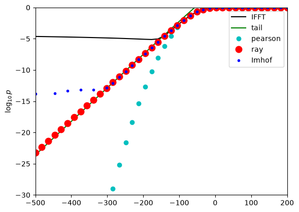
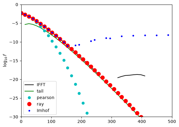
Ray, tail and Imhof methods are best for infinite tails.
Compute CDF in an infinite lower tail
w = [1, 2, -3, -4]
k = [6, 5, 4, 3]
l = [5, 10, 0, 0]
s = 10
m = -50

x = np.linspace(-500, 200, 40)

p_ifft = gx2.cdf(x, w, k, l, s, m, method='ifft', span=1e7, n_grid=int(1e7))
p_imhof = gx2.cdf(x, w, k, l, s, m, method='imhof', AbsTol=0, RelTol=1e-10)
p_ray = gx2.cdf(x, w, k, l, s, m, method='ray', n_rays=int(1e6))
p_pearson = gx2.cdf(x, w, k, l, s, m, method='pearson')  # pearson sucks

# tail approximation for lower tail. Mentioning 'lower' is needed here.
# For output values that are too small for double precision, it returns
# their log10 values, which are negative.
p_tail = gx2.cdf(x, w, k, l, s, m, side='lower', method='tail')
p_tail = np.asarray(p_tail, dtype=float)
# convert all output values to their log10
p_tail[p_tail > 0] = np.log10(p_tail[p_tail > 0])

# plot markers largest first, smallest last, so overlapping dots all stay visible
plt.figure()
plt.plot(x, np.log10(p_ifft), '-k', label='IFFT')
plt.plot(x, p_tail, '-g', label='tail')
plt.plot(x, np.log10(p_pearson), '.c', markersize=12, label='pearson')
plt.plot(x, np.log10(p_ray), 'or', markersize=9, label='ray')
plt.plot(x, np.log10(p_imhof), '.b', markersize=6, label='Imhof')
plt.axis([-5e2, 200, -30, 0])
plt.legend()
plt.ylabel(r'$\log_{10} p$')
plt.show()
Compute PDF in an infinite upper tail
x = np.linspace(0, 500, 40)

f_ifft = gx2.pdf(x, w, k, l, s, m, method='ifft', span=1e7, n_grid=int(1e7))
f_imhof = gx2.pdf(x, w, k, l, s, m, method='imhof', AbsTol=0, RelTol=1e-1)
f_ray = gx2.pdf(x, w, k, l, s, m, method='ray', n_rays=int(1e6))
f_pearson = gx2.pdf(x, w, k, l, s, m, method='pearson')

# tail approximation for upper tail. Mentioning 'upper' is needed here.
f_tail = gx2.pdf(x, w, k, l, s, m, side='upper', method='tail')

# plot markers largest first, smallest last, so overlapping dots all stay visible
plt.figure()
plt.plot(x, np.log10(f_ifft), '-k', label='IFFT')
plt.plot(x, np.log10(np.asarray(f_tail, float)), '-g', label='tail')
plt.plot(x, np.log10(f_pearson), '.c', markersize=12, label='pearson')
plt.plot(x, np.log10(f_ray), 'or', markersize=9, label='ray')
plt.plot(x, np.log10(f_imhof), '.b', markersize=6, label='Imhof')
plt.axis([0, 500, -30, 0])
plt.legend()
plt.ylabel(r'$\log_{10} f$')
plt.show()
Compute CDF in a finite lower tail
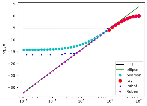
Ruben and ellipse methods are best for finite tails.
w = [1, 2, 3, 4]
k = [6, 5, 4, 3]
l = [5, 10, 0, 0]
s = 0
m = 0

x = np.logspace(-2, 2, 40)

p_ifft = gx2.cdf(x, w, k, l, s, m, method='ifft', span=1e7, n_grid=int(1e7))
p_imhof = gx2.cdf(x, w, k, l, s, m, method='imhof', AbsTol=0, RelTol=1e-10)
p_ruben = gx2.cdf(x, w, k, l, s, m, method='ruben')
p_ray = gx2.cdf(x, w, k, l, s, m, method='ray', n_rays=int(1e5))
p_pearson = gx2.cdf(x, w, k, l, s, m, method='pearson')
p_ellipse = gx2.cdf(x, w, k, l, s, m, method='ellipse')

# plot markers largest first, smallest last, so overlapping dots all stay visible
plt.figure()
plt.plot(x, np.log10(p_ifft), '-k', label='IFFT')
plt.plot(x, np.log10(np.asarray(p_ellipse, float)), '-g', label='ellipse')
plt.plot(x, np.log10(p_pearson), '.c', markersize=12, label='pearson')
plt.plot(x, np.log10(p_ray), 'or', markersize=9, label='ray')
plt.plot(x, np.log10(p_imhof), '.b', markersize=6, label='Imhof')
plt.plot(x, np.log10(p_ruben), 'om', markersize=4, label='Ruben')
plt.xscale('log')
plt.legend(loc='lower right')
plt.ylabel(r'$\log_{10} p$')
plt.show()
Distribution of quadratic form of a normal variable
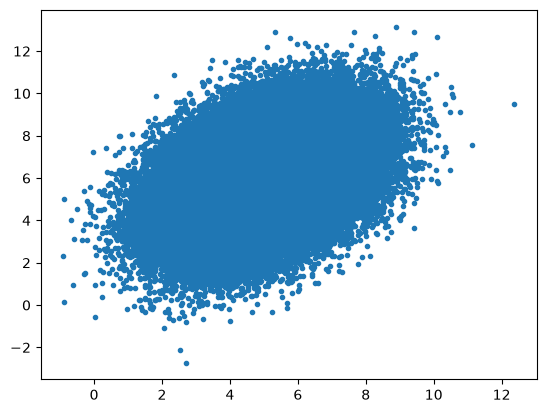
Normal parameters:
mu = np.array([5, 6])      # mean
v = np.array([[2, 1], [1, 3]])  # covariance matrix
Sample normal random vectors:
x = np.random.multivariate_normal(mu, v, int(1e5)).T
plt.figure()
plt.plot(x[0, :], x[1, :], '.')
plt.show()
Quadratic form $q(\mathbf{x})=(x_1+x_2)^2-x_1-1 = [x_1;x_2]',[1\ 1; 1\ 1],[x_1;x_2] + [-1;0]',[x_1;x_2] - 1$
quad = {'q2': np.array([[1, 1], [1, 1]]),
        'q1': np.array([-1, 0]),
        'q0': -1}
Compute the quadratic form q for the sample of normal vectors:
q = np.sum(x * (quad['q2'] @ x), axis=0) + quad['q1'] @ x + quad['q0']
Get generalized chi-square parameters corresponding to this quadratic form:
w, k, l, s, m = gx2.norm_quad_to_gx2_params(mu, v, quad)
print("w      =", w)
print("k      =", k)
print("l=", l)
print("s      =", s)
print("m      =", m)
w      = [7.]
k      = [1.]
l= [16.61880466]
s      = 0.8451542547285165
m      = -1.3316326530612201
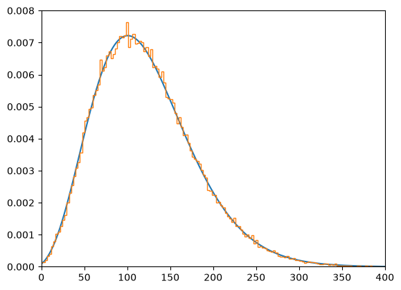
Compare the sampled and calculated distributions of q:
f, _, xf = gx2.pdf('full', w, k, l, s, m)
plt.figure()
plt.plot(xf, f)
plt.hist(q, bins=200, density=True, histtype='step')
plt.xlim([0, 400])
plt.show()
Compare the sampled and calculated means and variances:
mu_q, v_q = gx2.stat(w, k, l, s, m)
print([mu_q, q.mean()])
print([v_q, q.var()])
[122.0, np.float64(121.92202088814828)]
[3355.999999999998, np.float64(3324.8071301989507)]
Compare the sampled and calculated probabilities $p(q(\mathbf{x})<50)$:
print((q < 50).mean())
print(float(gx2.cdf(50, w, k, l, s, m)))
0.08404
0.08559335530030304
Find a canonical quadratic form of a standard multinormal corresponding to these generalized chi-square parameters:
quad = gx2.gx2_to_norm_quad_params(w, k, l, s, m)
print("q2 =\n", quad['q2'])
print("q1 =", quad['q1'])
print("q0 =", quad['q0'])
q2 =
 [[7. 0.]
 [0. 0.]]
q1 = [-57.07263542   0.84515425]
q0 = 115.0
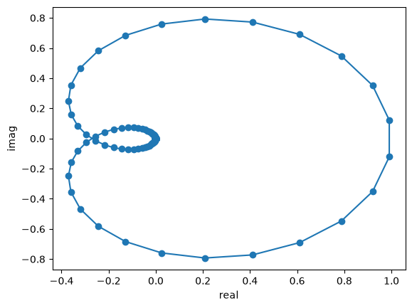
Compute characteristic function
t = np.linspace(-1, 1, int(1e3))
phi = gx2.char(t, w, k, l, s, m)
plt.figure()
plt.plot(phi.real, phi.imag, '-o')
plt.xlabel('real'); plt.ylabel('imag')
plt.show()
1st & 2nd derivatives (gradient & Hessian) of CDF wrt distribution parameters
This uses first and second derivatives computed analytically (faster and more accurate), than finite-differencing the cdf, which is slower and noisier.
Gradient and Hessian wrt the 'native' parameters
Take a generalized chi-square and a point $x_0$, and ask how the cdf $F(x_0)$ changes as we nudge the distribution parameters.
w = [1, -5, 2]
k = [1, 2, 3]
l = [2, 3, 7]
s = 2
m = 5
x0 = 10

# The gradient is a flat vector over all parameters, in the canonical order
# [w, k, l, s, m] (all of w, then all of k, ...); the Hessian is the
# matching square matrix.
grad, hess = gx2.cdf_grad_gx2(x0, w, k, l, s, m, hess=True)
print("grad =", grad.ravel())
print("hess shape =", hess.shape)
grad = [-5.93248766e-02 -6.46817998e-02 -1.83416585e-01 -2.03994081e-02
  9.33654797e-02 -4.02313224e-02 -2.01733664e-02  8.03252777e-02
 -3.89155815e-02  4.26856717e-05 -2.05327351e-02]
hess shape = (11, 11)
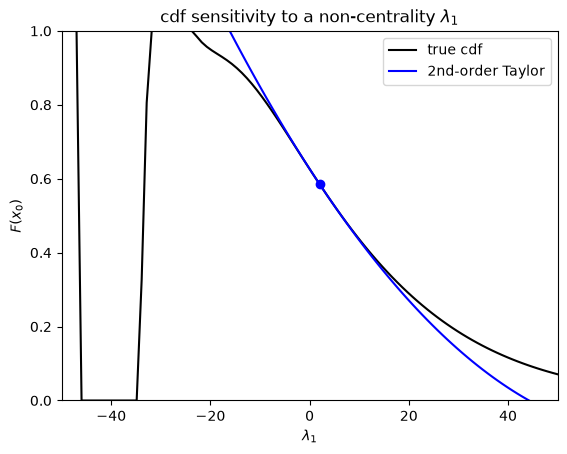
Taylor picture: vary one native parameter and predict the cdf
We compute derivatives only wrt $\lambda$, then use the first and second derivative of $\lambda_1$ to build the second-order Taylor model of $F(x_0)$ as $\lambda_1$ moves.
$F(x_0)$, $\frac{\partial F(x_0)}{\partial \lambda_1}$ and $\frac{\partial^2 F(x_0)}{\partial \lambda_1^2}$:
F0 = float(gx2.cdf(x0, w, k, l, s, m))
g, H = gx2.cdf_grad_gx2(x0, w, k, l, s, m, wrt=['l'], hess=True)
gl = g[0, 0]; Hl = H[0, 0]

delta = np.linspace(-50, 50, 100)
Ftrue = np.array([gx2.cdf(x0, w, k, np.array(l) + [d, 0, 0], s, m) for d in delta]).ravel()
Ftaylor = F0 + gl * delta + 0.5 * Hl * delta ** 2

plt.figure()
plt.plot(l[0] + delta, Ftrue, 'k-', label='true cdf')
plt.plot(l[0] + delta, Ftaylor, '-b', label='2nd-order Taylor')
plt.plot(l[0], F0, 'bo', markerfacecolor='b')
plt.xlabel(r'$\lambda_1$'); plt.ylabel('$F(x_0)$')
plt.axis([-50, 50, 0, 1])
plt.legend()
plt.title(r'cdf sensitivity to a non-centrality $\lambda_1$')
plt.show()
Gradient and Hessian wrt the parameters of the quadratic boundary
mu = np.array([1, 2])
v = np.array([[2, 1], [1, 3]])
quad = {'q2': np.array([[1, 1], [1, 1]]), 'q1': np.array([-1, 0]), 'q0': -1}
x0 = 0

grad, hess = gx2.cdf_grad_norm_quad(x0, mu, v, quad, hess=True)
print("dF/dQ2:\n", grad['q2'])
print("dF/dq1:", grad['q1'])
print(f"dF/dq0: {grad['q0']:.4f}")
dF/dQ2:
 [[-0.06275115  0.02888145]
 [ 0.02888145 -0.07839456]]
dF/dq1: [ 0.01277197 -0.05881688]
dF/dq0: -0.0962
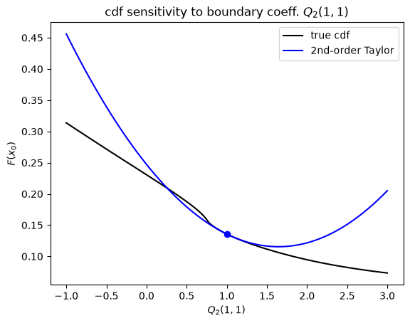
Taylor picture: vary one boundary parameter and predict the cdf
We compute the second-order Taylor approximation of $F(x_0)$ wrt variations in $\mathbf{Q}_{11}$.
$F(x_0)$, $\frac{\partial F(x_0)}{\partial Q_{11}}$ and $\frac{\partial^2 F(x_0)}{\partial Q_{11}^2}$:
w2, k2, l2, s2, m2 = gx2.norm_quad_to_gx2_params(mu, v, quad)
F0 = float(gx2.cdf(x0, w2, k2, l2, s2, m2))
g11 = grad['q2'][0, 0]; H11 = hess['q2q2'][0, 0, 0, 0]

# helper: probability with the Q2(1,1) coefficient perturbed by d
def probq(mu, v, quad, d, x0):
    q = {'q2': quad['q2'].astype(float).copy(), 'q1': quad['q1'], 'q0': quad['q0']}
    q['q2'][0, 0] += d
    w, k, l, s, m = gx2.norm_quad_to_gx2_params(mu, v, q)
    return float(gx2.cdf(x0, w, k, l, s, m))

delta = np.linspace(-2, 2, 100)
Ftrue = np.array([probq(mu, v, quad, d, x0) for d in delta])
Ftaylor = F0 + g11 * delta + 0.5 * H11 * delta ** 2

plt.figure()
plt.plot(quad['q2'][0, 0] + delta, Ftrue, 'k-', label='true cdf')
plt.plot(quad['q2'][0, 0] + delta, Ftaylor, '-b', label='2nd-order Taylor')
plt.plot(quad['q2'][0, 0], F0, 'bo', markerfacecolor='b')
plt.xlabel('$Q_2(1,1)$'); plt.ylabel('$F(x_0)$')
plt.legend()
plt.title('cdf sensitivity to boundary coeff. $Q_2(1,1)$')
plt.show()
Gradient and Hessian of classification error at the optimal boundary between two normal classes
Take two normal classes and find the quadratic (Bayes-optimal) boundary between them:
mu0, v0 = np.array([-.3, -.3]), np.array([[1., 0.], [0., 1.]])
mu1, v1 = np.array([.3, .3]), np.array([[.4, 0.], [0., .6]])
p0 = p1 = 0.5

# The optimal (Bayes) quadratic boundary q(x) = x'Q2 x + q1'x + q0 = 0
# between two normals (class 1 favored where q(x)>0)
quad = gx2.opt_norm_quad_bd(mu0, v0, mu1, v1, p0=p0, p1=p1)

def q(x, quad):
    return (np.einsum('i...,ij,j...->...', x, quad['q2'], x)
            + np.einsum('i,i...->...', quad['q1'], x) + quad['q0'])

def cov_ellipse(mu, v, n_std=1, n_pts=200):
    theta = np.linspace(0, 2 * np.pi, n_pts)
    circle = np.stack([np.cos(theta), np.sin(theta)])
    eigval, eigvec = np.linalg.eigh(v)
    return mu[:, None] + n_std * eigvec @ (np.sqrt(eigval)[:, None] * circle)

lim = 4
xs = np.linspace(-lim, lim, 400)
X1, X2 = np.meshgrid(xs, xs)
Q = q(np.stack([X1, X2]), quad)

plt.figure()
plt.plot(*cov_ellipse(mu0, v0), 'b-', label='class 0')
plt.plot(*cov_ellipse(mu1, v1), 'r-', label='class 1')
plt.contour(X1, X2, Q, levels=[0], colors='k')
plt.plot([], [], 'k-', label='optimal boundary')  # legend entry for the contour
plt.gca().set_aspect('equal')
plt.xlabel('$x_1$'); plt.ylabel('$x_2$')
plt.legend()
plt.show()
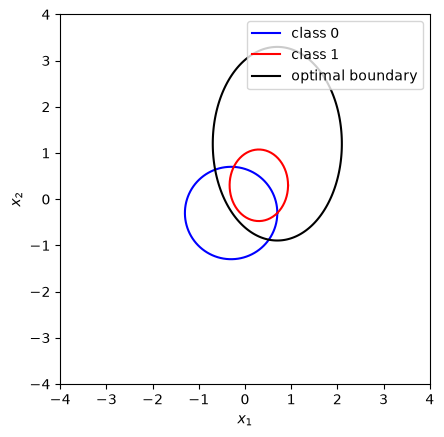
Compute the classification error, its gradient at this boundary (zero here, since the boundary is already optimal), and Hessian wrt the boundary coefficients:
err, grad, hess = gx2.norm_err(mu0, v0, mu1, v1, quad, p0=p0, p1=p1, hess=True)
print(f"classification error at the optimal boundary: {err:.4f}")
print("dE/dQ2 (~0):\n", grad['q2'])
print("dE/dq1 (~0):", grad['q1'])
print(f"dE/dq0 (~0): {grad['q0']:.2e}")

print()
print("Hessian blocks of the error wrt the boundary coefficients:")
print("d2E/dQ2^2:\n", hess['q2q2'])
print("d2E/dq1dQ2:\n", hess['q1q2'])
print("d2E/dq1^2:\n", hess['q1q1'])
print("d2E/dq0dq1:", hess['q0q1'])
print("d2E/dq0dQ2:\n", hess['q0q2'])
print(f"d2E/dq0^2: {hess['q0q0']:.4f}")
classification error at the optimal boundary: 0.2776
dE/dQ2 (~0):
 [[-1.38777878e-17  6.24500451e-17]
 [ 6.24500451e-17 -2.77555756e-17]]
dE/dq1 (~0): [-5.03069808e-17 -2.77555756e-17]
dE/dq0 (~0): -1.39e-17

Hessian blocks of the error wrt the boundary coefficients:
d2E/dQ2^2:
 [[[[ 0.10686131 -0.01406778]
   [-0.01406778  0.03496892]]

  [[-0.01406778 -0.00657552]
   [ 0.07651337 -0.02951635]]]


 [[[-0.01406778  0.07651337]
   [-0.00657552 -0.02951635]]

  [[ 0.03496892 -0.02951635]
   [-0.02951635  0.113363  ]]]]
d2E/dq1dQ2:
 [[[ 0.05454011  0.01426542]
  [-0.02135823  0.00439097]]

 [[-0.00354641 -0.02377665]
  [ 0.03255858  0.02350785]]]
d2E/dq1^2:
 [[ 0.06066359 -0.03275448]
 [-0.03275448  0.06589891]]
d2E/dq0dq1: [ 0.00791412 -0.02134665]
d2E/dq0dQ2:
 [[ 0.06066359 -0.03275448]
 [-0.03275448  0.06589891]]
d2E/dq0^2: 0.1237
1 maintainer

Download files
Download the file for your platform. If you're not sure which to choose, learn more about installing packages.
Source Distribution
Built Distribution
Filter files by name, interpreter, ABI, and platform.
If you're not sure about the file name format, learn more about wheel file names.
Copy a direct link to the current filters
File details
Details for the file gx2-1.2.tar.gz.
File metadata
- Download URL: gx2-1.2.tar.gz
- Upload date:
- Size: 894.1 kB
- Tags: Source
- Uploaded using Trusted Publishing? Yes
- Uploaded via:
twine/7.0.0 CPython/3.13.14
File hashes
| Algorithm | Hash digest | |
|---|---|---|
| SHA256 |
b52168587222d45d05e1b222dbc6e8f706923b8e10063895d1e1cdb5794d79fa
|
|
| MD5 |
0973a91eb7dfbb9ac2e01a8006d2cfed
|
|
| BLAKE2b-256 |
a8b374e68072103da1fe3f5cced27430bef9c106e54c99707cecac0d4f26f429
|
Provenance
The following attestation bundles were made for gx2-1.2.tar.gz:
Publisher:
publish.yml on abhranildas/gx2-py
-
Statement:
-
Statement type:
https://in-toto.io/Statement/v1 -
Predicate type:
https://docs.pypi.org/attestations/publish/v1 -
Subject name:
gx2-1.2.tar.gz -
Subject digest:
b52168587222d45d05e1b222dbc6e8f706923b8e10063895d1e1cdb5794d79fa - Sigstore transparency entry: 2313470213
- Sigstore integration time:
-
Permalink:
abhranildas/gx2-py@d4ca55e8f2e0128f440860e326084b186f0b97ca -
Branch / Tag:
refs/tags/v1.2 - Owner: https://github.com/abhranildas
-
Access:
public
-
Token Issuer:
https://token.actions.githubusercontent.com -
Runner Environment:
github-hosted -
Publication workflow:
publish.yml@d4ca55e8f2e0128f440860e326084b186f0b97ca -
Trigger Event:
release
-
Statement type:
File details
Details for the file gx2-1.2-py3-none-any.whl.
File metadata
- Download URL: gx2-1.2-py3-none-any.whl
- Upload date:
- Size: 51.2 kB
- Tags: Python 3
- Uploaded using Trusted Publishing? Yes
- Uploaded via:
twine/7.0.0 CPython/3.13.14
File hashes
| Algorithm | Hash digest | |
|---|---|---|
| SHA256 |
ad64e5231ab73384fba4c530cb961960390cf491baa7927dca1d36ac72f0b210
|
|
| MD5 |
dcb27b4bad4c363d5db5d9d4c97e154d
|
|
| BLAKE2b-256 |
54c8000a541aec920d095047c9d6fe91a98abb48a3a04d8ef1e396973c4f45c3
|
Provenance
The following attestation bundles were made for gx2-1.2-py3-none-any.whl:
Publisher:
publish.yml on abhranildas/gx2-py
-
Statement:
-
Statement type:
https://in-toto.io/Statement/v1 -
Predicate type:
https://docs.pypi.org/attestations/publish/v1 -
Subject name:
gx2-1.2-py3-none-any.whl -
Subject digest:
ad64e5231ab73384fba4c530cb961960390cf491baa7927dca1d36ac72f0b210 - Sigstore transparency entry: 2313470223
- Sigstore integration time:
-
Permalink:
abhranildas/gx2-py@d4ca55e8f2e0128f440860e326084b186f0b97ca -
Branch / Tag:
refs/tags/v1.2 - Owner: https://github.com/abhranildas
-
Access:
public
-
Token Issuer:
https://token.actions.githubusercontent.com -
Runner Environment:
github-hosted -
Publication workflow:
publish.yml@d4ca55e8f2e0128f440860e326084b186f0b97ca -
Trigger Event:
release
-
Statement type:














