
Fully-Differentiable Tensor Spherical Harmonics in JAX
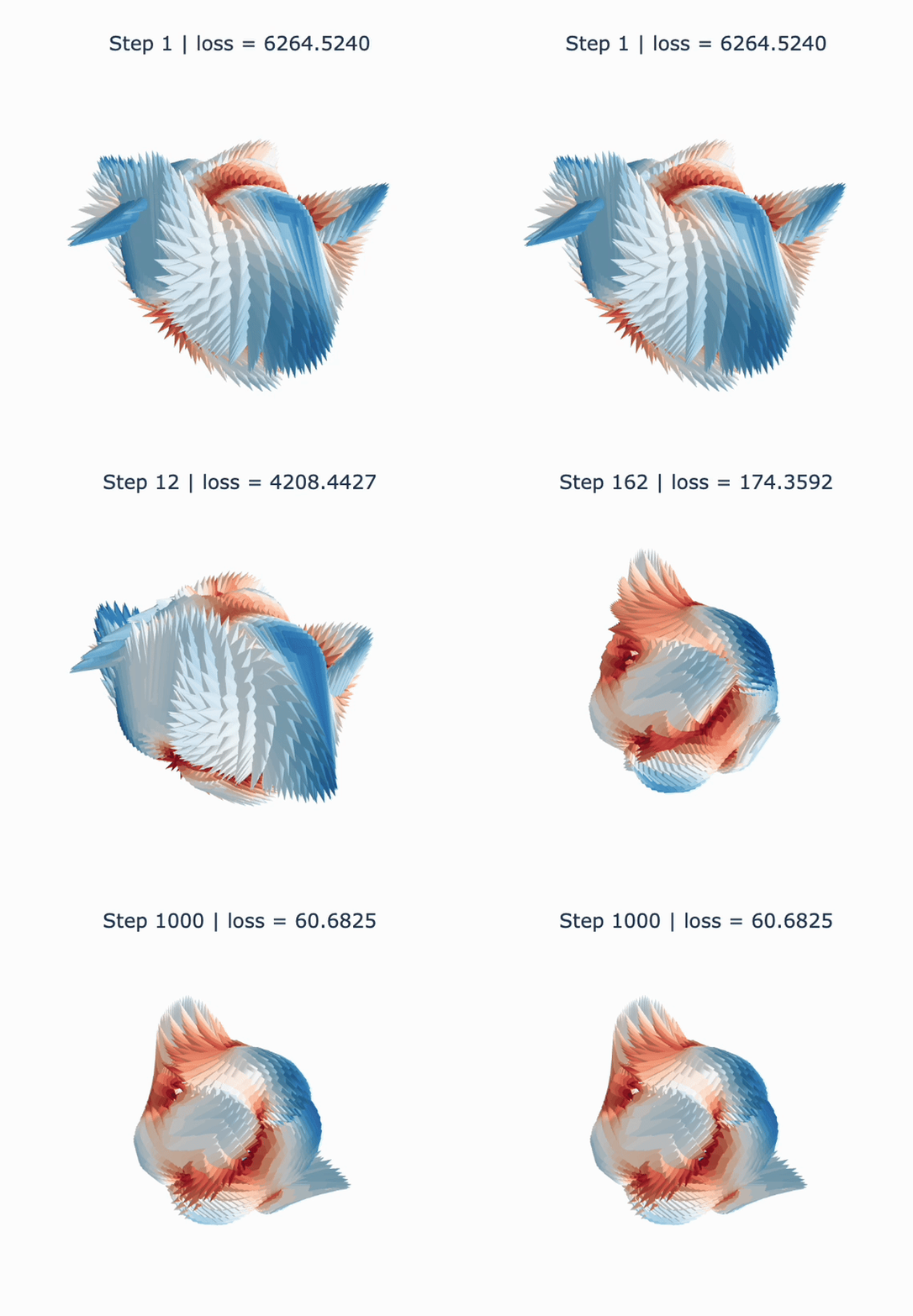
Fitting a tensor field from noisy scattered measurements via gradient descent on tensor spherical harmonic coefficients.
Here, we have implemented the tensor spherical harmonics in JAX, building on top of the e3nn-jax framework.
uv pip install harmonyx
Spherical irrep (or tensor) signals are functions defined on the sphere $S^2$ which map each point to a $SO(3)$ irrep of type $s$. We can imagine decomposing each component of the output giving $2s+1$ regular spherical harmonics. For each spherical harmonic degree $l$, we obtain a set of functions which transform as the tensor product rep $s \otimes l$ of $SO(3)$. By decomposing this tensor product rep into a direct sum of irreps (of type $j$), we obtain the definition of tensor spherical harmonics.
$$(Y_{j,m_j}^{\ell,s}){m_s}=\sum{m_\ell}C^{j,m_j}{\ell,m\ell,s,m_s}Y^{m_\ell}_{\ell}$$
Note: This library uses the e3nn-jax conventions for defining the spherical harmonics and irreps. Hence, the Clebsch-Gordan coefficients and resulting harmonics will differ slightly from those used in quantum physics. Our preprint and the symbolic checks in symbolic/ use the conventions defined in quantum physics.
The usual (scalar) spherical harmonics simply correspond to $s = 0$, as $0 \otimes l \equiv l$ and we can drop the redundant labels of $j$ and $m_s$.
Thus, the tensor spherical harmonics are a generalization of the spherical harmonics to arbitrary spin $s \geq 0$. To specify a tensor spherical harmonic, we must specify overal transformation type $j$, output irrep type $s$, and spherical harmonic degree $l$.
For example, to create the tensor spherical harmonic corresponding to $s = 2, l = 1, j = 2, m_j = 0$:
from harmonyx import TensorSphericalHarmonics
x = TensorSphericalHarmonics.tensor_spherical_harmonic(s=2, l=1, j=2, mj=0, parity=1)
Manipulating Tensor Spherical Harmonics
To obtain the coefficients of the tensor spherical harmonics from a tensor field:
x = TensorSphericalHarmonics.from_tensor_signal(
    tensor_signal, # e3nn.SphericalSignal with dimension [2s + 1, res_beta, res_alpha].
    s=2,
    lmax=10,
    parity=1
)
and to convert the coefficients back to a tensor field at a given resolution (here, a $100 \times 99$ Gauss-Legendre Grid):
tensor_signal = x.to_tensor_signal(
    res_beta=100,
    res_alpha=99,
    quadrature="gausslegendre"
)
If you only want to evaluate the tensor spherical harmonic coefficients at a given set of points, you can do:
points = jax.random.normal(jax.random.PRNGKey(0), shape=(10, 3))  # 10 random points
points = points / jnp.linalg.norm(points, axis=-1, keepdims=True)  # Normalize to lie on the sphere

values_at_points = x.at_points(points) # e3nn.IrrepsArray with shape [10, 2s + 1] containing the values of the tensor spherical harmonic at the given points.
To get the coefficient for a specific $(l, j, m_j)$ from the tensor spherical harmonic, you can use the get_coefficient method:
x = TensorSphericalHarmonics.normal(s=2, lmax=2, parity=1, key=jax.random.PRNGKey(0))
coefficient = x.get_coefficient(l=1, j=2, mj=0)
or to set the coefficient for a specific $(l, j, m_j)$:
x = TensorSphericalHarmonics.zeros(s=2, lmax=2, parity=1)
x = x.set_coefficient(l=1, j=2, mj=0, value=1.0)
Similarly, you can get or set all $(2j + 1)$ coefficients for a given $(l, j)$:
x = TensorSphericalHarmonics.normal(s=2, lmax=2, parity=1, key=jax.random.PRNGKey(0))
coefficients = x.get_coefficients(l=1, j=2)  # shape (2j + 1,) containing coefficients
x = x.set_coefficients(l=1, j=2, values=jnp.ones(2 * 2 + 1))  # set all coefficients for (l=1, j=2) to 1.0
Irrep Signal Tensor Product (ISTP)
Further, we have implemented the corresponding irrep signal tensor product (ISTP) which interacts two irrep (tensor) fields on the sphere with a pointwise tensor product. See our preprint to understand how the irrep signal tensor product enables faster Clebsch-Gordan tensor products.
x = TensorSphericalHarmonics.normal(s=2, lmax=2, parity=1, key=jax.random.PRNGKey(0))
y = TensorSphericalHarmonics.normal(s=2, lmax=2, parity=1, key=jax.random.PRNGKey(1))

z = x.reduce_pointwise_tensor_product(y, s_out=3, res_beta=100, res_alpha=99, quadrature="gausslegendre")
Plotting
To plot the tensor spherical harmonics as a 3D cone plot over $S^2$, you can do:
x.plot(dims=(0, 1, 2), res_beta=100, res_alpha=99, quadrature="gausslegendre")
Since we can only plot 3D vector fields, you need to specify the dims argument to indicate which three dimensions of the $SO(3)$ irrep to plot. For example, dims=(0, 1, 2) plots the first three dimensions of the irrep, while dims=(2, 3, 4) plots the last three dimensions of the irrep for $s = 2$.
This requires the plotly package, which you can install via uv pip install plotly 'nbformat>=4.2.0'.
To visualize the intensity (squared l2-norm of all $(2s + 1)$ entries at each point) of the tensor spherical harmonic on the sphere, you can do:
x.plot_intensity(res_beta=100, res_alpha=99, quadrature="gausslegendre")
Vector Spherical Harmonics
Our implementation directly leads to the vector spherical harmonics by simply setting $s = 1$:
from harmonyx import VectorSphericalHarmonics
x = VectorSphericalHarmonics.vector_spherical_harmonic(l=1, j=2, mj=0, parity=1)
as well as the corresponding vector signal tensor product (VSTP) which interacts two vector fields on the sphere:
x = VectorSphericalHarmonics.normal(lmax=2, parity=1, key=jax.random.PRNGKey(0))
y = VectorSphericalHarmonics.normal(lmax=2, parity=1, key=jax.random.PRNGKey(1))

z = x.reduce_pointwise_cross_product(y, res_beta=100, res_alpha=99, quadrature="gausslegendre")
All other methods described above for the tensor spherical harmonics are also available for the vector spherical harmonics.
See our example notebooks!
Citation
Please cite our preprint if you use this repository:
@misc{xie2026asymptoticallyfastclebschgordantensor,
  title={Asymptotically Fast Clebsch-Gordan Tensor Products with Vector Spherical Harmonics},
  author={YuQing Xie and Ameya Daigavane and Mit Kotak and Tess Smidt},
  year={2026},
  eprint={2602.21466},
  archivePrefix={arXiv},
  primaryClass={cs.LG},
  url={https://arxiv.org/abs/2602.21466},
}
1 maintainer

Metadata
1 maintainer
Release files for harmonyx 0.1.0
For a detailed explanation of source distributions (sdists) and built distributions (wheels), please see the package formats documentation.
Source distribution (sdist)
| File | Size | Uploaded | |
|---|---|---|---|
| harmonyx-0.1.0.tar.gz | 12.8 kB | Details |
Built distribution (wheel)
| File | Interpreter | ABI | Platform | Reset |
|---|---|---|---|---|
| harmonyx-0.1.0-py3-none-any.whl | Python 3 | none | any | Details |
Total release size: 22.4 kB
Release files / harmonyx-0.1.0.tar.gz
| Download URL | harmonyx-0.1.0.tar.gz |
|---|---|
| Size | 12.8 kB |
| Tags | Source |
|
SHA-256 checksum How to use checksums |
572695a1b4f47f346be6c7f4acbdfba15810111f6df47ad4a6a955b87705be07
|
|
BLAKE2b-256 checksum How to use checksums |
57226e3aab4ed8a516409cf855c2f1031e329c0a2dc1c1101ac2799474c0b49f
|
| Upload date | |
|
Uploaded using Trusted Publishing? What is trusted publishing? |
No |
| Uploaded via |
twine/6.2.0 CPython/3.11.13
|
Release files / harmonyx-0.1.0-py3-none-any.whl
| Download URL | harmonyx-0.1.0-py3-none-any.whl |
|---|---|
| Size | 9.6 kB |
| Tags | Python 3 |
|
SHA-256 checksum How to use checksums |
00b2efe525f05e20a1fadf47eda8739dd0da218bac1da9ea5948240b366be951
|
|
BLAKE2b-256 checksum How to use checksums |
03821ca62ba197120aee5c37912a555c662f0569dd5a9f122f707fc867298ae6
|
| Upload date | |
|
Uploaded using Trusted Publishing? What is trusted publishing? |
No |
| Uploaded via |
twine/6.2.0 CPython/3.11.13
|













