
hdfe-stream
Regression with several high-dimensional fixed effects, on data that does not
fit in memory: linear (feols_stream), and Poisson, logit and probit
(fepois_stream, feglm_stream).
from hdfe_stream import feols_stream

fit = feols_stream(
    "log_earn ~ age_squared + age_cubed | worker_id + firm_id + year",
    "data/*.parquet",              # a Parquet path or glob, never fully loaded
    workdir="scratch",             # where intermediates go: disk, not memory
    vcov={"CRV1": "worker_id"},
)
fit.summary()
Formulas follow pyfixest/fixest syntax and are parsed by pyfixest's own parser, so the syntax, the coefficient names and the results all match. The difference is where the work happens: rows are streamed off disk in batches and never held as a design matrix.
When to use this, and when not to
Use pyfixest. It is the better tool whenever your data fits in memory:
mature, broader in scope, more inference options, and no scratch directory to
think about. If a pandas DataFrame of your data fits comfortably in RAM, stop
reading.
Use this when it doesn't. The case it was built for is a matched employer–employee panel — tens of millions of rows, millions of worker effects, an AKM variance decomposition — on a machine or a secure enclave where the data is larger than the memory you are allowed. Concretely, reach for it when:
- the data does not fit in memory, or fits so tightly that nothing else does;
- you have one very high-cardinality dimension (workers, patients, students) whose groups each touch only a few levels of the others;
- you want worker-specific slopes as well as intercepts (
worker_id[t]), which multiplies the parameter count by the number of slopes; - the design is wide: hundreds of covariates, such as a categorical expanded into fine indicators or many interactions. An in-memory library needs rows × covariates in memory before it starts; this needs one batch of rows × covariates at a time, with any number of fixed effects, including one or none (see many covariates);
- you need a hard, predictable memory ceiling — a shared cluster, or a job that must not be the one that gets killed.
You are trading memory for disk, and you need scratch space: about five times
the size of your Parquet input while the fit runs, and only the result files
once it finishes. See benchmarks for what that buys. Point
workdir= at it, or set the HDFE_STREAM_WORKDIR environment variable once
(for example to a cluster's scratch filesystem) and leave workdir out; a
workdir passed to a call takes precedence, and with neither, the system
temporary directory is used.
How it works, in one paragraph
One fixed-effect dimension — normally the largest — is streamed: it
is never represented as a vector in memory. Every other dimension is held as a
vector sized by its number of levels, not rows. Rows are read in batches,
hash-partitioned into buckets by the streamed dimension, sorted one bucket at a
time, and reduced to a table of cells (one per combination of fixed-effect
levels). The reduced normal equations for the non-streamed dimensions are then
solved by conjugate gradient, and the streamed effects are recovered group by
group in a final pass that writes residuals and fixed effects straight to
Parquet. So memory scales with firms × years, not with workers × rows, and that
asymmetry is the whole design. The covariates travel with the rows: what is
held at once is one bucket or batch of rows × covariates, never all of them,
which is why a wide design fits where an in-memory one does not. Full detail is in
hdfe_stream/__init__.py.
Install
pip install hdfe-stream[formula] # formula syntax needs pyfixest
polars, numpy, numba, pyarrow and scipy are required. The extras:
| extra | what it adds |
|---|---|
formula |
feols_stream formula syntax and pyfixest reporting (pyfixest, formulaic, pandas) |
within |
the solver="within" backend |
amg |
algebraic multigrid preconditioning (precond="amg") for hard geometries |
all |
all of the above |
test |
the test suite |
Without formula you still get StreamingHDFE, the lower-level interface that
takes column names or Polars expressions instead of a formula string.
Features
Fixed effects. Any number of dimensions, including one (a within
regression, y ~ x | worker_id) and none (OLS with an intercept, y ~ x).
Interactions with ^
(firm_id^year). Varying slopes on the streamed dimension in fixest syntax
(worker_id[t], worker_id[t, t2]). Connected components of the
worker–firm graph are computed and reported, and the degrees-of-freedom
correction counts the fixed-effect parameters that are actually identified
(fe_dof="exact") or follows pyfixest's convention (fe_dof="pyfixest").
Covariates. Transformations (I(age**2), log(x)), categoricals (C(x),
string columns), interactions (:, *), event-study terms
(i(year, treat, ref=2009)). Terms spanned by the fixed effects are dropped
exactly as pyfixest drops them. Every term compiles to a Polars expression, so
the design is built while the data streams, one bucket at a time: a categorical
expanded into hundreds of indicators is carried through the partitioning as the
one column it comes from.
Standard errors. iid, heteroskedasticity-robust (hetero/HC1), and CRV1
clustered on any column, any ^ interaction, or several dimensions at once
(multi-way Cameron–Gelbach–Miller, any number of ways). Ask for several at fit
time with cluster= and switch between them afterwards with with_vcov() —
they are all computed in the one residual pass. CRV3, the cluster jackknife
(vcov={"CRV3": var}), for OLS when every fixed effect is nested within the
clusters or there are none; see limitations.
Estimators. OLS, weighted least squares (weights=, analytic or frequency),
and 2SLS (y ~ exog | fe | endog ~ instruments) with a first-stage F. Poisson
(fepois_stream, with an offset) and logit and probit (feglm_stream), with
weights; see below.
Multiple models. Several outcomes (y1 + y2 ~ ...), stepwise covariate sets
(sw(), csw()) and stepwise fixed-effect sets. Models sharing a fixed-effect
set share one pass over the data and one solve.
Leave-out variance components. The Kline–Saggio–Sølvsten bias correction for
the AKM decomposition, via leave_out_kss — including the leave-one-out
connected set, Johnson–Lindenstrauss leverages, weights, standard errors with
95% intervals (se=True), KSS's weak-identification diagnostic saying whether
those intervals are justified, and the interval that stays valid when they are
not. See below and
docs/kss.md.
Output. Coefficients as a Polars DataFrame (tidy()); the model-level
information of summary() (observations, fixed-effect counts, fit statistics,
solver) as JSON with summary_json(), optionally written to a file with
summary_json("fit.json") (summary_dict() returns the same as a dict);
residuals and
per-row fixed effects as lazy Polars scans, so aggregates like a variance
decomposition run as a streaming pass; estimated effects per dimension via
fixef(). to_pyfixest() converts a result into a pyfixest model for
pf.etable, pf.summary, pf.coefplot and pf.iplot, and hdfe_stream.etable
mixes streaming and in-memory models in one table.
Operations. Progress, warnings and summaries to a logging logger as they
happen. Each fit works in its own run directory; intermediates are deleted as
soon as they are no longer needed, everything is removed if the fit fails, and
hdfe_stream.cleanup() sweeps up after killed jobs.
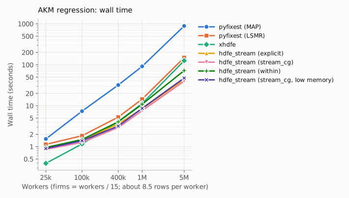
Benchmarks
A standard three-way AKM specification,
log_earn ~ age_squared + age_cubed | worker_id + firm_id + year, clustered by
worker, on the simulated panel that ships with the library. It is compared with
pyfixest, under both of its
demeaners, and with xhdfe, on its
CPU backend. Sizes run from 25,000 to 5,000,000 workers, with firms = workers /
15 at every size and about 8.5 rows per worker, so the largest panel has 42.5
million rows. Every configuration agrees with every other on the coefficients
to within 4e-10, so these are measurements of equally good answers. Reproduce
with:
pip install -e ".[benchmark]"      # xhdfe installs separately: see benchmarks/README.md
python benchmarks/akm_benchmark.py
python benchmarks/plot_benchmarks.py
The numbers behind the figures are in
benchmarks/results/akm.csv, and
benchmarks/README.md says how each is measured. In
brief: wall time includes reading the data, because pyfixest and xhdfe need it in
memory before they can start and hdfe_stream reads it itself — that difference is
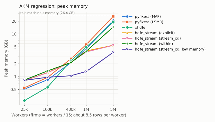
the comparison, not an artifact. Peak memory is VmHWM for the whole process,
including about 0.5 GB of imports. Each configuration runs in its own process.
At 5 million workers:
| configuration | wall time | peak memory | peak disk |
|---|---|---|---|
| pyfixest (MAP, its default) | 888 s | 20.7 GB | — |
| pyfixest (LSMR) | 150 s | 25.8 GB | — |
| xhdfe | 126 s | 19.1 GB | — |
hdfe_stream (stream_cg) |
40 s | 5.4 GB | 3.9 GB |
hdfe_stream (stream_cg, low memory) |
48 s | 3.7 GB | 4.0 GB |
Reading the figures
Memory is the point. At 5 million workers the in-memory libraries peak at
19–26 GB: pyfixest's LSMR run needed almost all of this machine's 26 GB.
hdfe_stream peaks at 5.4 GB with its defaults and 3.7 GB with the batch and
bucket sizes turned down ("low memory": rows_per_bucket=250_000,
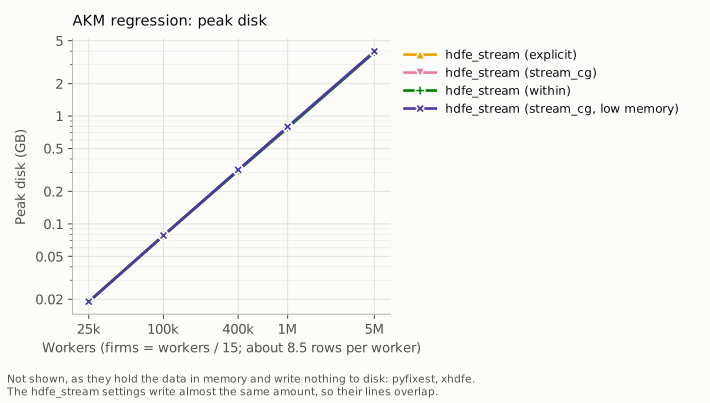
batch_rows=200_000), for about 20% more time and the same answer. What it
spends instead is disk: about 90 bytes per row, 4 GB at 42.5 million rows, freed
when the fit finishes. The in-memory libraries' peak grows in proportion to the
data. hdfe_stream's low-memory setting grows far more slowly: 0.8 GB at 25,000
workers, 1.3 GB at a million, 3.7 GB at five million.
It is not slower for it. From about 400,000 workers up, hdfe_stream is the fastest configuration measured. At 5 million workers it takes 40 s against xhdfe's 126 s and pyfixest's 150 s (LSMR) or 888 s (MAP). With AKM panel data, reducing rows to worker-firm cells before solving more than pays for the disk traffic. The simulated panel has about 8.5 rows per worker and one cell per row, which suits this approach; a specification where the cell table is no smaller than the data, and the fixed effects are less local, may do worse.
Below about 400,000 workers, the in-memory libraries use less memory. Running any hdfe_stream fit costs about 0.8 GB, most of it importing polars, numba and scipy and starting Polars' streaming engine and numba's thread pools. On small data that floor dominates: at 25,000 workers xhdfe peaks at 0.27 GB and pyfixest at about 0.5 GB. This is the concrete version of "use pyfixest (or xhdfe) if your data fits".
The default pyfixest demeaner is not the one to compare against.
MapDemeaner (alternating projections) is about 6x slower than LsmrDemeaner
from 400,000 workers up, since many worker effects are the case alternating
projections struggles with. If you are comparing, compare against LSMR.
hdfe_stream's within solver uses more memory at scale: 14.7 GB at 5
million workers, where stream_cg and explicit stay near 5.4 GB. Prefer
those when memory is the constraint.
Many covariates
The same kind of comparison, holding the data fixed and varying its width: the
million-worker panel (8.5 million rows, 66,665 firms) with age entered as
indicators, log_earn ~ i(age_bin) | worker_id + firm_id, clustered by worker,
in bins from five years wide (8 indicators) down to one month (503). hdfe_stream
runs at its defaults and "sized to the design", with bucket, batch and row-group
sizes scaled down as the design widens (the rule is below). The numbers are in
benchmarks/results/covariates.csv; every
configuration that finished agrees with every other to within 1e-8.
python benchmarks/covariates_benchmark.py
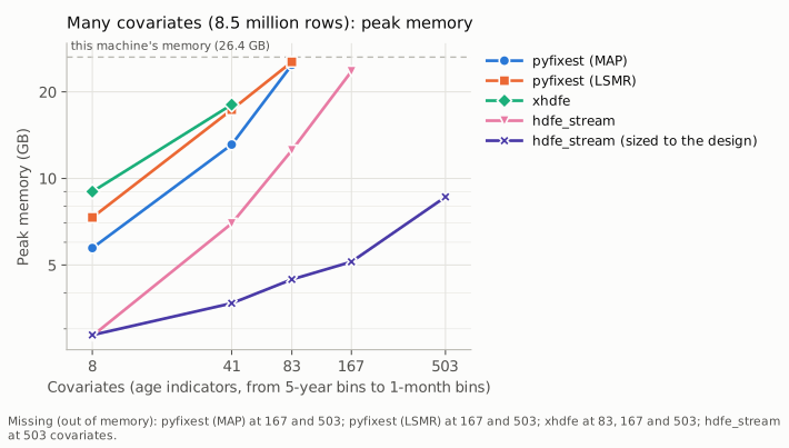
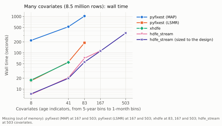
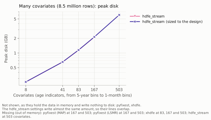
Wall time and peak memory ("—": ran out of this machine's 26 GB):
| covariates | pyfixest (MAP) | pyfixest (LSMR) | xhdfe | hdfe_stream | hdfe_stream, sized |
|---|---|---|---|---|---|
| 8 | 219 s, 5.7 GB | 17 s, 7.3 GB | 18 s, 9.0 GB | 7 s, 2.8 GB | 7 s, 2.9 GB |
| 41 | 522 s, 13.1 GB | 56 s, 17.3 GB | 55 s, 18.1 GB | 21 s, 7.0 GB | 20 s, 3.7 GB |
| 83 | 1,026 s, 24.8 GB | 189 s, 25.4 GB | — | 71 s, 12.5 GB | 56 s, 4.5 GB |
| 167 | — | — | — | 114 s, 23.6 GB | 112 s, 5.1 GB |
| 503 | — | — | — | — | 351 s, 8.6 GB |
The in-memory libraries run out first. Their peak grows with rows × covariates. At 8.5 million rows pyfixest was within 1 GB of this machine's 26 GB at 83 indicators and out of memory at 167; xhdfe was already out of memory at 83. hdfe_stream sized to the design goes from 2.9 GB at 8 indicators to 5.1 GB at 167 and 8.6 GB at 503. Of that last figure, about 4.9 GB is the memory-mapped cell table: file pages the kernel can drop under pressure. The memory the fit itself allocated peaked at 4.6 GB (a separate profile, reading the process's anonymous and file-backed pages apart).
Size the batches to the design. At its defaults hdfe_stream holds a whole
bucket of up to 20 million rows, with every covariate, while it sorts; that is
fine for a handful of covariates and not for hundreds (23.6 GB at 167, out of
memory at 503). Every step that holds rows holds all the covariates, so scale
rows_per_bucket, batch_rows and row_group_size down with the width. The
benchmark aims at about 1 GB of design per bucket and 250 MB per batch and row
group, never above the defaults:
per_row = 8 * (k + 4)                   # k covariates, plus outcome and ids
batch = min(2_000_000, int(250e6 // per_row))
fit = feols_stream(fml, data, rows_per_bucket=min(20_000_000, int(1e9 // per_row)),
                   batch_rows=batch, row_group_size=min(500_000, batch))
Time grows with the square of the width. The cross-products cost k × k per row; they are formed chunk by chunk as BLAS matrix products, and 503 indicators take 6 minutes where 167 take 2. hdfe_stream is the fastest configuration at every width measured.
Timings on this machine are noisy where memory is tight. Each point is one run. Repeated runs of the default configuration at 83 indicators, which holds 12.5 GB, took between 53 and 83 s; the sized configuration varied by about 15%. The differences between libraries above are far larger than that.
Disk grows with the width too, since the working copy of the rows carries every covariate: 0.3 GB at 8 indicators, 6 GB at 503.
How the design is built matters. A formula term such as i(age_bin) is
carried through the partitioning as the one column it is computed from, and the
indicators are built one bucket at a time. That works for any expression whose
value on a row depends on that row alone, which formula terms always do. With
the low-level StreamingHDFE, an expression that needs the whole column
(pl.col("x") - pl.col("x").mean(), a window, a shift) is detected and the design
is built before partitioning instead, with a warning: the estimates are the
same, the memory is not. Define such a column in the input LazyFrame to avoid
it. result.diagnostics["design_evaluated"] says which happened.
examples/wide_designs.py puts this together.
Trading memory for time
Same data, same solver, same answer — only how much is in flight at once:
python benchmarks/akm_benchmark.py --memory-sweep 1000000
8,500,353 rows, 1,000,000 worker effects
rows_per_bucket |
batch_rows |
wall time | peak memory | peak disk |
|---|---|---|---|---|
| 20,000,000 (default) | 2,000,000 | 7.1 s | 3,861 MB | 779 MB |
| 1,000,000 | 500,000 | 7.4 s | 1,560 MB | 781 MB |
| 250,000 | 200,000 | 7.8 s | 1,343 MB | 795 MB |
| 100,000 | 100,000 | 9.3 s | 1,280 MB | 789 MB |
Most of the saving comes from the first step down. The defaults are tuned for a
machine with room to spare; if memory is the binding constraint, set
rows_per_bucket to something near what you can afford and leave the rest
alone (with many covariates, scale batch_rows and row_group_size down too;
see many covariates). rhs_block bounds the other big
array (levels × variables), and
max_s_gb caps the explicit reduced matrix, above which solver="auto" falls
back to stream_cg by itself.
Leave-out estimation has a memory knob of its own, scratch_mb; see
docs/kss.md.
Measured on an Intel Core Ultra 7 258V, 8 cores, 26 GB RAM, Linux (WSL2); Python 3.13.5, polars 1.44.2, numpy 2.5.3, numba 0.67.0, scipy 1.18.1, pyfixest 0.60.0, xhdfe 2.28.0 (CPU backend). The exact versions are in benchmarks/results/machine.json. Numba kernels are compiled on first use and cached to disk; the benchmark runs a warm-up fit so compilation is not charged to any configuration.
Choosing a solver
solver |
what it does | when |
|---|---|---|
"auto" (default) |
explicit, falling back to stream_cg if the reduced matrix would exceed max_s_gb |
leave it alone |
"explicit" |
builds the reduced matrix once and solves it in memory | fastest when it fits; its size depends on how levels co-occur, not on rows |
"stream_cg" |
applies the reduced matrix by streaming the cell table each iteration | when the reduced matrix is the thing that does not fit |
"within" |
hands the reduced system to within-py |
an alternative; no varying-slopes support |
The streamed dimension is chosen for you: an explicit stream= if given, else
the dimension carrying varying slopes, else the highest approximate cardinality.
result.diagnostics["stream"] says which and why.
Examples
Runnable, on simulated data, no setup — see examples/:
quickstart.py |
fit a model and read the results |
akm_variance.py |
the variance decomposition, in a streaming pass |
formulas.py |
the formula syntax, end to end |
weights_and_iv.py |
weights and 2SLS |
fewer_fixed_effects.py |
one fixed effect, or none |
glm.py |
Poisson with an offset, logit and probit, separation, and the incidental parameter bias |
wide_designs.py |
hundreds of covariates, and sizing the batches to them |
varying_slopes.py |
worker-specific trends, and the low-level interface |
out_of_core.py |
memory, disk, solvers, logging |
reporting.py |
tables and plots via pyfixest |
leave_out_kss.py |
the KSS bias correction, checked against the effects the data was built from |
Simulated data
hdfe_stream.simulate ships with the package, so you can try the library, or
check your own code, against data whose answer you know:
from hdfe_stream.simulate import simulate_akm

simulate_akm(n_workers=1_000_000).write_parquet("sim.parquet")
simulate_akm draws worker and firm effects explicitly and positively assorted,
with enough mobility to connect the firms into one component. simulate_rich
adds categoricals, non-fixed-effect cluster variables, weights, an IV block and
missing values; simulate_trends adds worker-specific time trends. All are
deterministic given a seed.
Poisson, logit and probit
from hdfe_stream import fepois_stream, feglm_stream

pois = fepois_stream("visits ~ x | worker_id + firm_id + year", "data/*.parquet",
                     offset="log_exposure", workdir="scratch")
logit = feglm_stream("promoted ~ x | firm_id + year", "data/*.parquet", "logit",
                     workdir="scratch")
These are fitted by iteratively reweighted least squares, each step a weighted version of the linear regression above. Pass 0 sorts the rows once. Each step then reads them once, rebuilding every row's linear predictor from the current coefficients, and solves the reduced system, starting from the previous step's solution.
Nothing row-sized is rewritten between steps, so the disk needed is about what OLS needs. A fit takes a few times as long as OLS on the same data, since it usually needs 6 to 10 steps. Benchmarks against pyfixest, over the AKM benchmark's panel sizes and over the number of covariates, are in docs/glm.md.
Fixed-effect levels whose effect would be infinite are dropped first: all-zero outcomes for Poisson, constant ones for logit and probit. Estimates, standard errors and deviance match pyfixest to about 1e-12. The few places where they deliberately differ are frequency weights, which here mean repeated rows, and logit and probit levels whose outcome is all 1, which are dropped. Both are described in docs/glm.md, along with the options and results.
Leave-out variance components (KSS)
The plug-in AKM decomposition is biased: worker and firm effects are estimated
with error, which inflates their variances and attenuates their covariance.
leave_out_kss applies the bias correction of
Kline, Saggio and Sølvsten (2020), streaming
like the rest of the package:
from hdfe_stream import leave_out_kss

lo = leave_out_kss("log_earn ~ age_squared | worker_id + firm_id",
                   "data/*.parquet", workdir="scratch", se=True)
print(lo.summary())
It follows Saggio's reference implementation, LeaveOutTwoWay. It prunes to the leave-one-out connected set, leaves out a worker–firm match by default, and approximates leverages by random projection. It supports weights, standard errors, and KSS's weak-identification diagnostic and q = 1 interval.
docs/kss.md covers the options, the standard errors and their measured coverage, weak identification, validation, reproducibility, and performance against xhdfe: at 5 million workers, 5.3 GB of memory against xhdfe's 20 GB, with standard errors in 46 minutes where xhdfe's did not finish in three hours. docs/kss_methodological_differences.md lists every way this implementation differs from LeaveOutTwoWay, VarianceComponentsHDFE.jl, xhdfe and pytwoway, with the motivation and measured effect of each.
Reproducibility
Everything in a fit is deterministic: the same data and the same options give the same numbers, with no random component anywhere — to floating-point rounding. Repeated fits normally agree bit for bit, but aggregation runs in parallel, and once, under heavy CPU load from another process, two identical fits differed in the last digit. Treat agreement to about 1e-12 as the guarantee, not bitwise identity.
The exception is leave-out estimation, which uses random projection and random draws. Its results are reproducible from the seed but not deterministic; docs/kss.md says exactly what they depend on and what to report in a paper.
Correctness
The test suite checks every feature against pyfixest on simulated data —
coefficients, standard errors under each vcov, residuals, fixed effects, fit
statistics, the sample kept after dropping missing values, and the exact set of
coefficient names and dropped collinear terms. Varying slopes have no pyfixest
equivalent, so they are checked against a brute-force regression with explicit
worker-by-slope dummies; three-way clustering is checked against an
inclusion–exclusion sum built from pyfixest's own score matrix. Poisson, logit
and probit are checked against pyfixest's fepois and feglm, and their
frequency weights against pyfixest on the data with each row repeated.
pip install -e ".[test]"
pytest
Limitations
- Varying slopes only on the streamed dimension, and only one dimension may carry them.
- CRV3 only with nested fixed effects. The cluster jackknife is computed by downdating the fit, which is exact when every fixed effect is nested within the clusters (worker effects clustered by worker, firm × year effects by firm) or there are none. With fixed effects that are not nested, as in an AKM model clustered by worker, the jackknife has to re-estimate the fixed effects once per cluster, and the fit refuses; use CRV1, or pyfixest, which refits. CRV3 is also one-way and OLS only (pyfixest has no IV CRV3 either). No CRV2 and no wild bootstrap.
- Poisson, logit and probit: no CRV3, IV, varying slopes or leave-out
estimation; no detection of separation by the covariates (pyfixest's
"ir"check), only by the fixed effects; and no correction for the incidental parameter bias of logit and probit with fixed effects estimated from few observations, as in pyfixest and fixest. During the iterations the streamed dimension's effects are held in memory, one float per group per coefficient set. See docs/glm.md. - A converted result cannot recompute its own vcov, because it holds no
data. Ask for what you need at fit time via
cluster=. - Formula support pins a pyfixest range (
>=0.50,<0.61), because it uses pyfixest's internal formula modules.StreamingHDFEhas no such dependency. - Needs scratch disk, roughly the size of your data during the fit. Leave-out estimation adds to that: it memory-maps its row-sized accumulators rather than holding them, which is what keeps it inside a bounded memory footprint, at about 90 bytes per row of scratch while it runs.
- Wide designs need the batch sizes scaled down (see many covariates): the defaults hold a whole bucket of rows with every covariate. And the cross-products cost k × k per row, so time grows with the square of the number of covariates.
- Leave-out estimation handles one outcome at a time, and its standard errors omit the split-sample refinement of KSS §4.2 (so they are conservative, as their Lemma 5 provides for). Under weak identification it supplies the q = 1 interval, not KSS's q > 1 generalization. Leaving out a match, as it does by default, var(alpha) has no standard error and the covariance no q = 1 interval. See docs/kss.md.
1 maintainer

Metadata
1 maintainer
Release files for hdfe-stream 0.1.0
For a detailed explanation of source distributions (sdists) and built distributions (wheels), please see the package formats documentation.
Source distribution (sdist)
| File | Size | Uploaded | |
|---|---|---|---|
| hdfe_stream-0.1.0.tar.gz | 349.3 kB | Details |
Built distribution (wheel)
| File | Interpreter | ABI | Platform | Reset |
|---|---|---|---|---|
| hdfe_stream-0.1.0-py3-none-any.whl | Python 3 | none | any | Details |
Total release size: 513.7 kB
Release files / hdfe_stream-0.1.0.tar.gz
| Download URL | hdfe_stream-0.1.0.tar.gz |
|---|---|
| Size | 349.3 kB |
| Tags | Source |
|
SHA-256 checksum How to use checksums |
1c432d82d228ad117f4d4599737cc3a520c761e058f9202b4f237678c62e922c
|
|
BLAKE2b-256 checksum How to use checksums |
57220dc22113d79ef82a29acb4d58064a8149366cefe25762ad551f5914d3e90
|
| Upload date | |
|
Uploaded using Trusted Publishing? What is trusted publishing? |
Yes |
| Uploaded via |
twine/7.0.0 CPython/3.13.14
|
Provenance
Provenance describes where a file came from. On PyPI, provenance is shared via attestations, which provide a verifiable record of the build or publishing details. View details, limitations and caveats.


PyPI Publish Attestation
PyPI verified that this artifact, at this checksum, originated from the publisher listed below.
Signed by GitHub Actions, verified by PyPI on Oct 1, 2026.
Transparency logRelease files / hdfe_stream-0.1.0-py3-none-any.whl
| Download URL | hdfe_stream-0.1.0-py3-none-any.whl |
|---|---|
| Size | 164.4 kB |
| Tags | Python 3 |
|
SHA-256 checksum How to use checksums |
57c405751f7ffbccaa1865eb7df439ee43bcba6bc92e67c15cd5a206dde98a36
|
|
BLAKE2b-256 checksum How to use checksums |
fdd79572420d09fdbcd4a29e24715ab08d2133b5b992d28ed45a3055d0ccf767
|
| Upload date | |
|
Uploaded using Trusted Publishing? What is trusted publishing? |
Yes |
| Uploaded via |
twine/7.0.0 CPython/3.13.14
|
Provenance
Provenance describes where a file came from. On PyPI, provenance is shared via attestations, which provide a verifiable record of the build or publishing details. View details, limitations and caveats.
PyPI Publish Attestation
PyPI verified that this artifact, at this checksum, originated from the publisher listed below.
Signed by GitHub Actions, verified by PyPI on Oct 1, 2026.
Transparency log












