

Heatfall
Turn coordinate lists into clear maps colored by count.
Geohash rectangles or H3 cells · Legends built in · Pillow images and SVG maps
Quick start · Choose a grid · Color guide · Full documentation




Heatfall groups geographic observations into geohash rectangles or H3 cells, counts the points in each cell, and draws the occupied cells over a basemap. Save the result as a Pillow image, or combine a heat layer with points, routes, and service areas through Landfall.
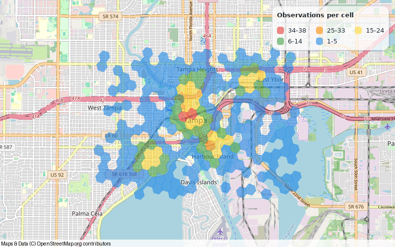
A seeded set of 1,040 synthetic observations, clustered around five Tampa
neighborhoods with scattered background activity. The default legend labels
each cell color with the point-count range it represents. Regenerate it with
examples/generate_doc_maps.py.
| Two grid systems | Counts stay explicit | Compose and export |
|---|---|---|
| Geohash rectangles or mostly-hexagonal H3 cells. | Raw counts named in built-in legends. | Add points and routes; export images or SVG. |
Install
Python 3.8–3.13 is supported. Install the latest published release with:
python -m pip install heatfall
New in 1.2.0: Translucent count legends are enabled by default. Place and style them precisely, use a sequential palette, or share explicit count colors across maps. See the release notes.
To install this release exactly:
python -m pip install "heatfall==1.2.0"
The examples below use Heatfall 1.2.0 or newer. Check your version with
python -m pip show heatfall.
The default OpenStreetMap basemap needs network access when tiles are not cached. No API key is required for that default provider.
Quick start
Create an H3 map from 15 synthetic observations. Repeated coordinates deliberately produce cells with different counts.
import heatfall

lats = [27.9470] * 8 + [27.9515] * 4 + [27.9430] * 2 + [27.9475]
lons = [-82.4580] * 8 + [-82.4500] * 4 + [-82.4475] * 2 + [-82.4400]

image = heatfall.plot_heat_h3s(
    lats,
    lons,
    precision=8,
    color_scheme="wheel",
    size=(800, 500),
)
image.save("h3-heatmap.png")
Both plotting functions return a PIL.Image.Image. Heatfall fits the map to the
added cells automatically. size is the output width and height in pixels.
For dataframe columns, pass lists such as df["latitude"].tolist() and
df["longitude"].tolist(). See the
point data guide for CSV
input and coordinate conversion.
Choose a grid
| Geohash | H3 | |
|---|---|---|
| Function | plot_heat_hashes() |
plot_heat_h3s() |
| Cell shape | Latitude/longitude rectangles | Mostly hexagons, with pentagons in the global grid |
precision range |
1–12 | 0–15; H3 calls this resolution |
| Choose it when | Your data or downstream tools already use geohashes | You want hexagonal aggregation or already use H3 |
| City-scale starting point | Try precision=6 |
Try precision=8 |
Higher precision means smaller cells. If most occupied cells contain only one point, reduce precision to aggregate more observations. Start with a coarser grid for data spread over a large region. The two precision scales are independent: geohash precision 8 and H3 resolution 8 do not imply the same cell size.
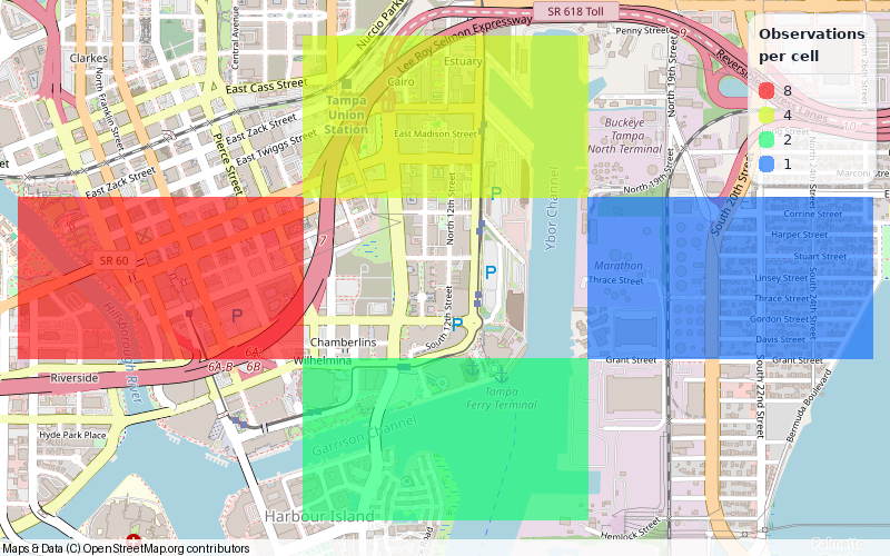
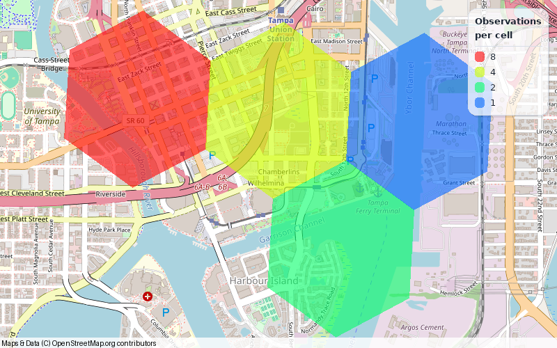
Geohash at precision 6, then H3 at resolution 8. The same 15 observations from the quick start appear in both grids. Each map fits its own cell boundaries, so the basemap extent can differ.
Create the same map using geohash cells:
import heatfall

lats = [27.9470] * 8 + [27.9515] * 4 + [27.9430] * 2 + [27.9475]
lons = [-82.4580] * 8 + [-82.4500] * 4 + [-82.4475] * 2 + [-82.4400]

image = heatfall.plot_heat_hashes(
    lats, lons, precision=6, color_scheme="wheel", size=(800, 500)
)
image.save("geohash-heatmap.png")
Understand the colors
Each observation contributes one count to its cell. Only occupied cells are drawn. Within a heat layer, cells with the same count share a color; different count levels receive different palette colors.
Heat fills default to 60% opacity (40% transparent), keeping streets and
labels visible beneath the cells. Set opacity on either plotting function or
heat layer method to control the fill: 0.4 is lighter, 1.0 is solid, and 0.0
is invisible. Opacity applies uniformly to the layer; counts still determine
the palette colors.
color_scheme |
Behavior |
|---|---|
"heatmap" — default |
Maps low-to-high counts to five steps from blue, green, yellow, orange, to red |
"distinct" |
Generates visually distinct colors for the count levels |
"wheel" |
Selects colors from an HSV color wheel |
"random" |
Generates random colors for the count levels |
"sequential" |
Maps lower counts to light blue and higher counts to dark blue |
The "heatmap" and "sequential" palettes order colors by numeric count; the
heatmap uses five color steps from blue at the low end through green, yellow,
and orange to red at the high end. Colors are scaled separately for each layer.
"distinct", "wheel",
and "random" distinguish count levels without implying an order, and
"distinct" and "random" may change between calls. Use count_colors to
assign fixed colors to count values when comparing maps.
The example below uses a sequential palette. For direct geohash/H3 comparisons, the shared color example fixes colors by count.
Legends are enabled by default. Their softly translucent panel lets heat cells
remain visible beneath the labels. The default heatmap legend has at most five
swatches, one for each palette color, labeled with the count range that color
represents. Other color schemes show each distinct count. Entries are discrete,
not a continuous gradient. Set legend=False to hide the legend. Use
heatfall.LegendOptions to style the title,
layer headings, labels, swatches, panel, and shadow independently, and to
control columns, count order, and exact placement. It lists high-to-low by
default; set count_order="ascending" for low-to-high. A map context also exposes immutable
context.heat_layers metadata and context.set_legend() for composed maps.
Use LegendOptions(background_color="white", background_opacity=0.65) for a
more transparent card. Background opacity ranges from 0 to 1 and multiplies
the color's existing alpha; text and swatches keep their own opacity. Set
shadow=False to remove the shadow as well.
Titles wrap by default to keep the card compact. Use title_max_width to set
the wrapping width in pixels, title_line_spacing to adjust wrapped line
spacing, or title_wrap=False to disable automatic wrapping. See the
placement and sizing gallery and
background opacity preview.
image = heatfall.plot_heat_h3s(
    lats, lons, precision=8,
    color_scheme="sequential",
    legend=heatfall.LegendOptions(
        position=(0.96, 0.08),
        units="fraction",
        anchor="top-right",
        offset=(-8, 8),
        title="Observations per cell",
    ),
)
Positions can use nine named anchors or any (x, y) coordinate in pixels or
fractions of the output dimensions. Placement is checked against the output
canvas; use allow_clipping=True only when intentional. The result shows raw
counts per cell, not counts normalized by cell area. It does not apply smoothing
or accept observation weights.
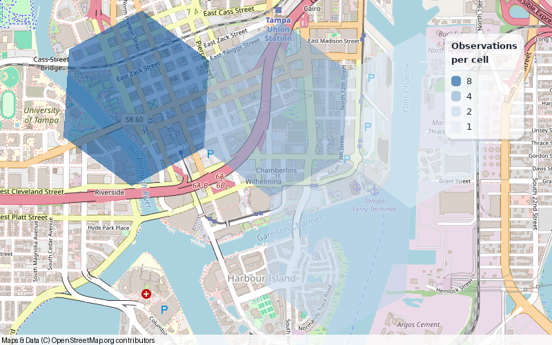
A sequential palette makes increasing counts read from light to dark blue. The legend's background is translucent; text and swatches retain their own opacity.
Add other layers
heatfall.Context extends landfall.Context, so heat cells can share a map with
ordinary geographic objects. Add the heat layer first, then add the overlays.
Landfall's Context API documents the inherited methods; its shapes and styling guide explains point sizes, line widths, circle radii, and overlay colors.
import heatfall

lats = [27.9470] * 8 + [27.9515] * 4 + [27.9430] * 2 + [27.9475]
lons = [-82.4580] * 8 + [-82.4500] * 4 + [-82.4475] * 2 + [-82.4400]

context = heatfall.Context()
context.add_heat_h3s(lats, lons, precision=8, color_scheme="wheel")

# A reference location.
context.add_points([27.9470], [-82.4580], colors=["black"], point_size=10)

# A route in (latitude, longitude) order.
context.add_line(
    [(27.9430, -82.4475), (27.9475, -82.4400)], color="black", width=3
)

# One circle per center, with radii in meters.
context.add_circles(
    [27.9515], [-82.4500], [300],
    color="blue", fill_color="transparent", width=2,
)

context.render_pillow(800, 500).save("layered-heatmap.png")
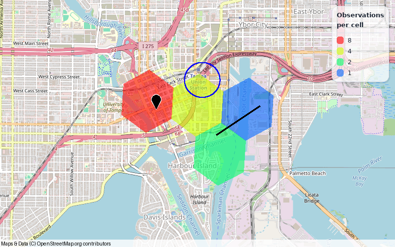
Landfall also supplies polygons, GeoJSON support, styling, and SVG rendering. See its documentation for the inherited methods. For Heatfall's own layer methods, see the API below. The image shows the 15-observation example above, including its default count legend.
API
The full API reference documents signatures, defaults, return values, and context heat methods.
The public package exports two plotting functions, Context, and the
LegendOptions and HeatLayerInfo types for configuring and inspecting legends:
| Entry point | Result |
|---|---|
heatfall.plot_heat_hashes() |
A Pillow image containing a geohash heat layer |
heatfall.plot_heat_h3s() |
A Pillow image containing an H3 heat layer |
heatfall.Context() |
A map context for composing layers |
Both plotting functions accept the same arguments:
| Argument | Default | Meaning |
|---|---|---|
lats |
Required | List of latitudes in decimal degrees, from −90 to 90 |
lons |
Required | Matching list of longitudes in decimal degrees, from −180 to 180 |
precision |
Required | Geohash length 1–12, or H3 resolution 0–15 |
color_scheme |
"heatmap" |
"heatmap", "distinct", "random", "wheel", or "sequential" |
tileprovider |
OpenStreetMap | A staticmaps.TileProvider for the basemap |
size |
(800, 500) |
Output (width, height) in pixels |
opacity |
0.6 |
Keyword-only fill opacity from 0.0 to 1.0 |
legend |
True |
Keyword-only; False, True, or LegendOptions |
count_colors |
None |
Keyword-only mapping of positive counts to fixed colors |
The heat layer methods mutate the context and return None; they also accept
keyword-only legend_label and count_colors. The context legend is enabled
by default, and set_legend(False) disables it:
context.add_heat_hashes(lats, lons, precision, color_scheme="heatmap", opacity=0.6)
context.add_heat_h3s(lats, lons, precision, color_scheme="heatmap", opacity=0.6)
context.set_legend(False)
The default provider is staticmaps.tile_provider_OSM.
Configure a context's basemap with context.set_tile_provider(provider) and
render it with context.render_pillow(width, height). The standalone plotting
keyword is spelled tileprovider, without an underscore.
See Landfall's custom tile service guide
for basemap configuration and its
SVG example
for exporting a composed map.
Input rules
- Supply parallel coordinate lists in latitude, longitude order, using decimal degrees. GeoJSON positions commonly use the reverse order.
- Lists must have matching lengths. Out-of-range coordinates and non-finite
values such as
NaNand infinity raiseValueError. - Use an integer precision in the supported range and one of the named palettes.
- Opacity must be finite and between
0.0and1.0, inclusive. - Standalone plotting functions reject empty lists. Adding an empty heat layer
to a
Contextis a no-op; add some content before rendering. - Repeated coordinates count as repeated observations. Deduplicate your input first if your analysis should count unique locations instead.
Crossing the antimeridian
H3 maps can contain points on both sides of ±180° longitude:
import heatfall

image = heatfall.plot_heat_h3s(
    lats=[10.0, 10.0, 10.0],
    lons=[179.5, -179.5, 179.5],
    precision=3,
)
image.save("antimeridian.png")
Heatfall splits crossing H3 cell boundaries into closed polygons at the
antimeridian, with intersections calculated along spherical edges. Both pieces
keep the original cell's observation count and color, and the automatic map
extent follows the short span across the seam. Exact 180 and -180 longitude
are accepted. These fixes require Heatfall 1.1.0 or newer.
This handling applies to rendered H3 cells. Polygon-to-cell filling of external GeoJSON is outside Heatfall's point API. For polar cells, H3 rendering is clipped to the Web Mercator tile latitude limit of approximately ±85.0511°; these maps do not display the poles.
See geographic considerations for coordinate rules, antimeridian behavior, and polar limits.
Documentation
Read the full documentation on Read the Docs. It includes a visual example gallery, a heat-colored light/dark theme, searchable guides, and an API reference generated from the package.
| Guide | What you will find |
|---|---|
| Getting started | Installation, coordinates, and your first image |
| Usage and styling | Grid choices, palettes, transparency, and layers |
| Point data | CSV input, coordinate pairs, and count semantics |
| Basemaps and output | Providers, fixed views, rendering without tiles, and SVG |
| Geography | Antimeridian handling and polar limits |
| Troubleshooting | Common errors and reproducible bug reports |
| API reference | Function signatures, defaults, and context heat methods |
| Development | Local checks, documentation builds, and contributing |
| Releasing | Compatibility notes and trusted publishing |
Troubleshooting
| Symptom | What to check |
|---|---|
| Every cell has the same color | Counts may all be equal. Use a coarser precision if you want more aggregation. |
| Cells appear in the wrong place | Check latitude/longitude order and decimal-degree units. For H3, use Heatfall 1.1.0 or newer. |
| Cells are larger or smaller than expected | Geohash and H3 use different precision scales. Adjust within the range for your chosen grid. |
| Basemap tiles are missing or rendering stalls | Check network access and tile-provider availability. Cached tiles can avoid later requests. |
| Colors differ between runs or maps | Palettes are generated per layer. Distinct and random colors can vary, and the number of count levels changes the palette. |
add_circles() raises TypeError |
Pass latitude, longitude, and radii sequences; use [1000] * len(lats) for equal one-kilometer radii. |
Keep the provider attribution visible when sharing map images. Heatfall's MIT license covers the package; basemap imagery has its own provider terms.
Develop and contribute
Create a virtual environment, then install the package with its development tools:
git clone https://github.com/eddiethedean/heatfall.git
cd heatfall
python -m venv .venv
Activate it with source .venv/bin/activate on macOS/Linux, or
.venv\Scripts\Activate.ps1 in Windows PowerShell. Then run:
python -m pip install -e ".[dev]"
python -m pytest
python -m tox -e ruff,mypy
pytest generates coverage reports. Ordinary rendering tests use mock tiles;
tests explicitly marked integration may make real tile requests.
To run the complete Python version matrix, install the matching interpreters and
run python -m tox. For a single installed version, use python -m tox -e py311.
CI runs tests on Python 3.8–3.13 on Linux, Python 3.13 on macOS and Windows, and
checks formatting, linting, types, and package builds.
Build the documentation
Use Python 3.12 or newer for Sphinx and the documentation dependencies:
python -m pip install -e ".[docs]"
python -m sphinx -b html -W --keep-going docs docs/_build/html
Open docs/_build/html/index.html to view the site. With Python 3.13 available,
python -m tox -e docs builds it in an isolated environment. CI also builds the
documentation and fails on warnings.
The published documentation builds through .readthedocs.yaml. See the
documentation development guide
for build tools and theme customization.
The README images are actual package output. Reproduce them with:
python examples/generate_doc_maps.py
The generator uses synthetic data and real OpenStreetMap tiles. It needs network access when those tiles are not already cached.
For changes, include a runnable example or a regression test where appropriate, run the checks above, and open a pull request. For bug reports, include your Python and Heatfall versions, a small coordinate sample, the precision, and the traceback.
Maintainers can follow the release guide
for compatibility notes, distribution validation, and publishing steps. Pushing
a matching vX.Y.Z tag runs the release checks and publishes to PyPI through
trusted publishing.
Dependencies and license
Heatfall uses Landfall ≥0.4.2 for map composition and colors, Geodude ≥0.1.1 and PyGeodesy for geohashes, and H3 ≥4.0.0 for H3 cells. Landfall provides the underlying py-staticmaps and Pillow rendering dependencies.
Released under the MIT license. Report bugs and request features in GitHub Issues.
1 maintainer

Metadata
1 maintainer
Release files for heatfall 1.2.0
For a detailed explanation of source distributions (sdists) and built distributions (wheels), please see the package formats documentation.
Source distribution (sdist)
| File | Size | Uploaded | |
|---|---|---|---|
| heatfall-1.2.0.tar.gz | 10.0 MB | Details |
Built distribution (wheel)
| File | Interpreter | ABI | Platform | Reset |
|---|---|---|---|---|
| heatfall-1.2.0-py3-none-any.whl | Python 3 | none | any | Details |
Total release size: 10.7 MB
Release files / heatfall-1.2.0.tar.gz
| Download URL | heatfall-1.2.0.tar.gz |
|---|---|
| Size | 10.0 MB |
| Tags | Source |
|
SHA-256 checksum How to use checksums |
27c7bd021abe5a096a2ad1cdf44fdd334aeb61526dc195f4d1a9516e8804247a
|
|
BLAKE2b-256 checksum How to use checksums |
3dec3c9030bcd1da69a542d9bacb87cee5fdc4ea41e422d8d38e783b9f8840c8
|
| Upload date | |
|
Uploaded using Trusted Publishing? What is trusted publishing? |
Yes |
| Uploaded via |
twine/7.0.0 CPython/3.13.14
|
Provenance
Provenance describes where a file came from. On PyPI, provenance is shared via attestations, which provide a verifiable record of the build or publishing details. View details, limitations and caveats.


PyPI Publish Attestation
PyPI verified that this artifact, at this checksum, originated from the publisher listed below.
Signed by GitHub Actions, verified by PyPI on Oct 5, 2026.
Transparency logRelease files / heatfall-1.2.0-py3-none-any.whl
| Download URL | heatfall-1.2.0-py3-none-any.whl |
|---|---|
| Size | 760.4 kB |
| Tags | Python 3 |
|
SHA-256 checksum How to use checksums |
57d3a95302e51cff6e085d318ea25fffa374d22aceb98fb0a0fb8c225d03ce6a
|
|
BLAKE2b-256 checksum How to use checksums |
f5623963217dbefe04208f231462893b4d33ae05290b7eeb31095cf1906b5d12
|
| Upload date | |
|
Uploaded using Trusted Publishing? What is trusted publishing? |
Yes |
| Uploaded via |
twine/7.0.0 CPython/3.13.14
|
Provenance
Provenance describes where a file came from. On PyPI, provenance is shared via attestations, which provide a verifiable record of the build or publishing details. View details, limitations and caveats.
PyPI Publish Attestation
PyPI verified that this artifact, at this checksum, originated from the publisher listed below.
Signed by GitHub Actions, verified by PyPI on Oct 5, 2026.
Transparency log
















