
Spatial crime analysis with hexagons and street segments

Project description
hexseg
hexseg is a Python package designed to simplify generating statistics to prioritise location for crime prevention efforts. It assists in streamlining two popular count-based methods by creating hexagonal grids or street-segment analyses across geographic study areas. It is designed with crime analysis in mind, but may also be suitable for other urban planning and resource allocation tasks.
Features
- Hexagonal grid analyses: generate Uber hexagon layers over a defined study area and calculate count and weight based statistics to identify and prioritise locations.
- Hexagonal grid statistics: calculate spatially lagged statistics (mean or sum of neighbours), generate global and local ranks and z-scores.
- Road segment analysis: calculate counts and ranks for road segments, or for contiguous clusters of segments, to identify and prioritise locations.
- Interactive visualisation: add priority hexagons and/or segments to interactive maps using folium.
Installation
Install via pip:
pip install hexseg
Alternatively, install directly from GitHub:
pip install git+https://github.com/routineactivity/hexseg.git
Quick Start
Here is an example to get started quickly
Hexagon Grid Example
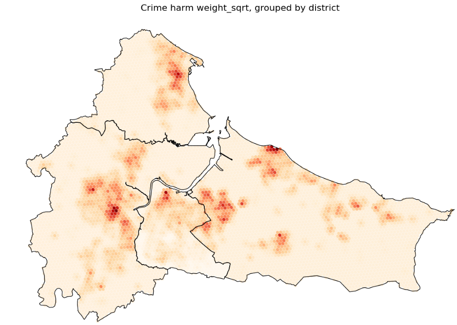
In this example, you can produce a range of count and weight statistics to prioritise places within hexagons.
import geopandas as gpd
import hexseg as HS

# filepaths
base = "https://raw.githubusercontent.com/routineactivity/hexseg/main/data"
districts = f"{base}/cleveland_districts.gpkg"
roads     = f"{base}/cleveland_roads.gpkg"
crimes    = f"{base}/cleveland_sample_data.gpkg"

gdf_districts = gpd.read_file(districts)
gdf_roads     = gpd.read_file(roads)
gdf_crimes    = gpd.read_file(crimes)

# generate hexagons for study boundaries
hexes = HS.get_hexagons(gdf_districts, name_col="lad21nm", resolution=9)

# summarise crime counts and/or weights from crime data to hexagons
hex_both = HS.summarise_by_hex(
    hexes_gdf=hexes,
    crimes_gdf=gdf_crimes,
    count_col='any',
    weight_col='pseudo_harm'
    )

# optional: add spatial lagged means/sums to counts/weights for nearest neighbours
# default neighbours is 6 - typically a 'donut' around hexagons, unless on edge of boundary
hex_lagged = HS.add_spatial_lag(
    hexes_gdf=hex_both,
    count_col='crime_count',
    weight_col='crime_weight',
    k=6
)

# add zscores and ranks (global and local) to measure/s being used for prioritisation
hex_stats = HS.add_spatial_stats(hex_lagged, col='weight_plus_mean_sqrt', group_col='geo_boundary')
Plotting Hexagon results
# Choose which measure you want to map outputs for
# Example below, the top 20 ranked by crime harm weight plus mean, grouped by district
# By this measure, we have selected the top 20 hexagons for each district
m = HS.create_folium_map(
      hex_gdf=hex_stats,
      hex_query="weight_plus_mean_sqrt_rank_by_geo_boundary <= 20",
      seg_gdf=None,
      seg_query=None,
      district_gdf=gdf_districts,
      district_query=None)
m

Street Segment Example
In this example, you can calculate crime counts for individual street segments or contiguous clusters of segments for easier prioritisation. Counting by individual segments alone often identifies more locations than can realistically be addressed with available resources. By clustering segments, you can create manageable areas for targeted interventions, customised based on segment size (reflecting patrol distance or officer coverage) and crime thresholds. Segment clusters can be used independently or combined with hexagonal grids to highlight priority streets within key hexagons.
import geopandas as gpd
import hexseg as HS

# filepaths
base = "https://raw.githubusercontent.com/routineactivity/hexseg/main/data"
districts = f"{base}/bkn_precincts.gpkg"
roads     = f"{base}/bkn_roads_lion.gpkg"
crimes    = f"{base}/bkn_sample_data.gpkg"

gdf_districts = gpd.read_file(districts)
gdf_roads     = gpd.read_file(roads)
gdf_crimes    = gpd.read_file(crimes)

# summarise number of crimes by segment
roads_with_counts = HS.count_crimes_by_nearest_road(
    crimes_gdf=gdf_crimes,
    roads_gdf=gdf_roads,
    max_dist=75 # set maximum distance from segment to point
    )

# build adjacency graph
G = HS.build_adj_graph(roads_with_counts,
                          fid_col=None,
                          crime_count_col='crime_count')

# create user defined clusters of segments
clusters = HS.segment_clusters(G, min_size=5, max_size=8, min_crimes=100)

# add cluster id and sum of crime in clusters to segment layer
gdf_clusters = HS.clusters_to_gdf(clusters, G, roads_with_counts, fid_col='fid', crime_count_col='crime_count')
Plotting segment results
# visualise results
# Visualise the street segment clusters
m = HS.create_folium_map(
      hex_gdf=None,
      hex_query=None,
      seg_gdf=gdf_clusters,
      seg_query="cluster_crime_sum > 200",
      district_gdf=gdf_districts,
      district_query=None)

m

# or visualise highest individual segments

# If you don't want to cluster segments and just see the highest
# Use the roads_with_counts object you created
m = HS.create_folium_map(
      hex_gdf=None,
      hex_query=None,
      seg_gdf=roads_with_counts,
      seg_query="crime_count > 20",
      district_gdf=gdf_districts,
      district_query=None)

m

Use Cases
- Public Safety: Identify and statistically rank places to prioritise police resource allocation.
- Urban Planning: Understand distributions of other datasets for planning purposes, where point data is available (i.e. education, social care, employment, public health)
Contributing
Contributions are welcome! This project is maintained as a hobby, so while issues and pull requests are appreciated, responses may be delayed.
Acknowledgements
This project was inspired by Madison-PD’s micro-time hotspots. ChatGPT helped translate previous workflows into reusable code and assisted with PyPI publication.
Release history Release notifications | RSS feed


Download files
Download the file for your platform. If you're not sure which to choose, learn more about installing packages.
Source Distribution
Built Distribution
Filter files by name, interpreter, ABI, and platform.
If you're not sure about the file name format, learn more about wheel file names.
Copy a direct link to the current filters
File details
Details for the file hexseg-0.1.3.tar.gz.
File metadata
- Download URL: hexseg-0.1.3.tar.gz
- Upload date:
- Size: 13.0 kB
- Tags: Source
- Uploaded using Trusted Publishing? No
- Uploaded via: twine/6.1.0 CPython/3.12.0
File hashes
| Algorithm | Hash digest | |
|---|---|---|
| SHA256 |
68bce6ffb677fbeeadd9bdfcd7c2d806c6c94106a15a07acbfc8d68627f92819
|
|
| MD5 |
664b78af28c457bde3d440dc9fd24ba7
|
|
| BLAKE2b-256 |
43fe878e05c7955f30abba802129cdde93d1107a1a0f7eb52d6d7fc50aea48d0
|
File details
Details for the file hexseg-0.1.3-py3-none-any.whl.
File metadata
- Download URL: hexseg-0.1.3-py3-none-any.whl
- Upload date:
- Size: 11.1 kB
- Tags: Python 3
- Uploaded using Trusted Publishing? No
- Uploaded via: twine/6.1.0 CPython/3.12.0
File hashes
| Algorithm | Hash digest | |
|---|---|---|
| SHA256 |
de5e903843059ac5fc37a6d19a48794651ff005ec735dd2da594e36350e2f619
|
|
| MD5 |
5a2c2b6a6b75821992e1f87b6aaa760c
|
|
| BLAKE2b-256 |
b8d87b1e380b516e1c705dc04885905407401f4835ecadee2f32b43785727cc9
|






