hidden-py 1.2.0

A python package for discrete-output hidden Markov models

A Hidden Markov Model package for python

Installation

To install this package simply run the command:

pip install hidden-py

Table of Contents

• Overview
  • Dynamics/Simulation
  • System Identification
  • Signal Processing
• Roadmap
• References

---

Overview

This package contains logic for inferring, simulating, and fitting Hidden Markov Models with discrete states and observations. This package serves as a complement to several common HMM packages that deal primarily with mixture models, where output symbols are continuous, and drawn from a distribution of values that is somehow conditional on the hidden state.

Here, we have considered scenarios where the observation value is an integer, and one of the possible hidden states, although this is not required, there could be more hidden states than possible observations, or vice-versa, all that really matters is that the observation values (and hidden state values) are discrete. There are three major use-cases for this codebase: dynamics/simulation, system identification/parameter fitting, and signal processing. In all cases, these functionalities are outlined in several tutorial notebooks in the notebooks/tutorials location of the github repository

Hidden Markov Models

Markov Models are a class of stochastic models for characterizing the behaviour of systems that transition between states randomly, with a probability that depends only on the current state of the system (i.e. they are memoryless). Because of this simplification, the dynamics on a set of discrete states can be captured entirely by a single matrix, known as the transition matrix, $A$, with elements $A_{ij} = p(x_t=i | x_{t-1} = j)$ quantifying the probability that during timestep $t-1 \to t$, the system will transition from state $j\to i$. Because of the normalization of probability, the columns of $A$ are constrained to be equal to unity.

Without any ambiguity in the observed value (i.e. the underlying Markov model is directly observed) the system is just a Markov model. The causal diagram of a Markov model is shown in the figure below.

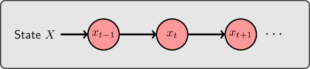
Here, the state $x_t$ at time $t$ only depends on the state at the previous time $t-1$. As a result the evolution of a probability distribution over states can be modelled by simply multiplying an initial distribution by the transition matrix, and repeating the process for each time step. For example, given an initial distribution over states at time 0 and a transition matrix $A$, the probability distribution at time $T$ is

$$ p_T = A^T \cdot p_0 $$

A hidden Markov model (HMM), on the other hand, is a probabilistic function of a Markov model. This means that the output of an HMM (the observation $y$) is correlated with the underlying (hidden/unobserved) state of the Markov model, but not necessarily equal to it. For a set of discrete possible observations (as we capture in this package), the observation process can also be modelled by a matrix (the observation matrix) $B$ with elements $B_{ij} = p(y_t = i | x_{t} = j)$ quantifying the probability that our measurement/observation $y_t$ at time $t$ is equal to $i$ given the hidden system is in state $j$. Here, the diagonal elements represent our probability of observing the correct state, while off-diagonals represent the probability of error. In comparison to the figure used in the Markov system, the below diagram shows how causality works in a hidden Markov model.

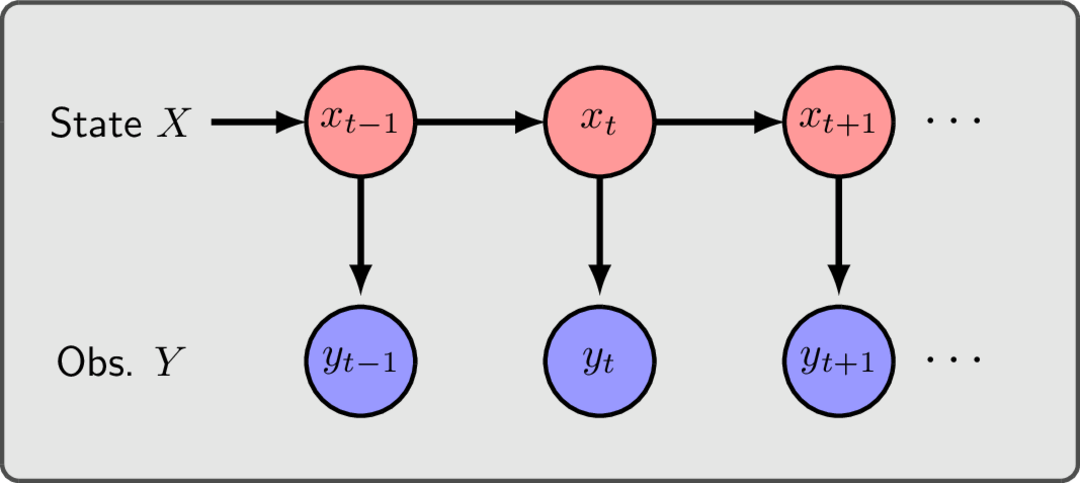
Here, the observations ($y_t$) are stochastic (random) functions of the underlying state, but not necessarily equal to it. However (importantly) the observation at time $t$ only depends explicitly on the hiddenstate at time $t$.

---

As for the components of the package, the goal of the simulation functionality is simply to generate trajectories of both the hidden state and observation time-series that are conistent with these probabilities. Conversely, the goal for system identification/parameter fitting is to find the most likely parameters (elements of the $A$ and $B$) matrices, given only a time series of observations. Finally, the goal if signal processing is to make use of the observation sequence (and a particular set of $A$ and $B$ matrices) to infer what the hidden state is at a particular point in time in a singl etime series.

Dynamics/Simulation

The hidden.dynamics submodule contains the code necessary to simulate the hidden state and observation dynamics as specified by a state transition matrix $A$ (with elements that quantify the rate of transitions between states) and an observation matrix $B$, with elements that quantify the probability of observing a given output symbol, given the current hidden state.

For instance, the code necessary to initialize a hidden Markov model, run the dyanamics, and extract the observation and state time-series

import hidden_py as hp

# 2 hidden states, 2 possible observation values
hmm = hp.dynamics.HMM(2, 2)

# Helper routine to initialize A and B matrices
hmm.init_uniform_cycle()

# Run dynamics for 100 time steps
hmm.run_dynamics(100)

# Pull out the observations, and true (simulated) hidden state values
observations = hmm.obs_ts
hidden_states = hmm.state_ts

As an example, the schematic below shows a possible trajectory for a HMM with 2 hidden states and 2 possible observation values.

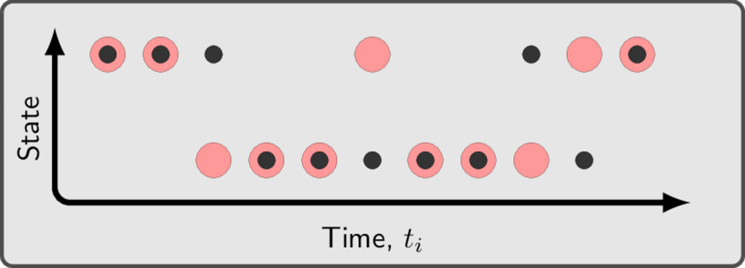
Here the red dots represent the state of the hidden system over time, while the black dots indicate the observed value at that point in time. So, at time point 3, for instance, the observed value differs from the hidden state. See the notebooks/tutorials/02-hidden-markov-model.ipynb in the github source for a more in-depth review of this process.

---

System Identification

The infer submodule contains the code that wraps lower-level functionality (primarily in the filters/bayesian.py and optimize/optimization.py files) for both signal processing and system identification/parameter fitting.

There are two separate approaches to perform system identification: Local/Global partial likelihood optimization, and complete-data likelihood optimization. While more comprehensive details are contained in the github notebooks, broadly speaking partial data likelihood optimization performs relatively standard optimizations on the likelihood function $\mathcal{L}(\theta | Y)$ which considers only the observations as the data. Effectively, these optimizers wrap the scipy.opt.minimize functions by encoding and decoding the $A$ and $B$ matrices into a parameter vector (ensuring that their column-normalization is preserved) and calculating the negative log-likelihood of a particular parameter vector. In practice, given a set of observations, we can initialize an analyzer and run either local (using, by default, the scipy.opt.minimize function with the SQSLP algorithm) or global (using the scipy SHGO algorithm) as:

import hidden_py as hp

# Input the dimensions of the HMM and observations
analyzer = hp.infer.MarkovInfer(2, 2)

# Initial estimates of the A and B matrices
A_est = np.array([
    [0.8, 0.1],
    [0.2, 0.9]
])

B_est = np.array([
    [0.9, 0.05],
    [0.1, 0.95]
])

# Run local partial-data likelihood optimization (default behaviour), the symmetric keyword can be used to specify whether or not the A and B matrices are assumed to be symmetric, and here, the opt_type of hp.OptClass.Local is used by default
opt_local = analyzer.optimize(observations, A_est, B_est, symmetric=False)

# And the partial-data global likelihood optimization, the A and B initial matrices are not used in the optimizer, aside from providing a way of specifying the dimension of the parameter vectors
opt_global = analyzer.optimize(observations, A_est, B_est, symmetric=False, opt_type=hp.OptClass.Global)

Now, for the complete-data likeihood optimization, the interface is very similar, but behind the scenes the code will run an implementation of the Baum-Welch reparameterization algorithm (an instance of an Expectation-Maximization algorithm) to find the optimal parameter values. In practice, this can be done as:

import hidden_py as hp

analyzer = hp.infer.MarkovInfer(2, 2)

res_bw = analyzer.optimize(observations, A_est, B_est, opt_type=hp.OptClass.ExpMax)

In all cases, there is also the ability to add algorithm options to customize the specifics of the optimization. Most relevant is for the expectation-maximization where you can specify a maximum number of iterations for the algorithm, as well as a threshold on the size of parameter changes (quantified by the matrix norm of pre- and post-update $A$ and $B$ matrices). This can be accessed through the algo_opts dictionary. For instance, if we wanted to change the maximum iterations in the BW algorithm to 1000 and set the termination threshold at 1e-10, we would perform the previous call as

options = {
    'maxiter': 1000,
    "threshold": 1e-10
}

res_bw = analyzer.optimize(observations, A_est, B_est, opt_type=hp.OptClass.ExpMax, algo_opts=options)

In essence, this set of tools allows you to infer the best model given a set of observed data. Under the hood, many of the tools from the signal processing module are used, but the analyzer.optimize(...) function calls largely hide that complexity.

---

Signal Processing

The infer submodule can also be used for the purposes of signal processing: given a valid estimate of the model parameters, how can we best estimate the hidden state value, given the observations. There are two distinct domains of application, first would be prediction in real time, where only observations in the past are available for inferring the current hidden state (this would use the so-called forward-filtered estimate). There is also an ex post approach, which uses the entirety of observations from a given period of time to estimate the hidden state at a particular point within that time period. This is the so-called Bayesian smoothed estimate of the hidden state.

Mathematically, if we denote $Y^t \equiv { y_0, y_1, \cdots, y_t }$ as the sequence of observations from tie $t=0$ up to time $t$, then for a total trajectory length of $T$, the forward filter and Bayesian smoothed estimate are calculating

$$ p(x_t | Y^t) \quad \to \qquad \text{Forward-filter} $$

$$ p(x_t | Y^T) \quad \to \quad \text{Bayesian smoother} $$

where, $x_t$ is the hidden state at time $t$.

Quantitatively the forward filter and Bayesian smoothed estimates of a given HMM sequence of observations can be calculated in the following way:

import hidden_py as hp

analyzer = hp.infer.MarkovInfer(2, 2)

# Gets the forward algorithm results
analyzer.forward_algo(observations, A, B)

# Gets the Bayesian-smoothed estimate of the hidden state
analyzer.bayesian_smooth(observations, A, B)

The tutorial notebook notebooks/tutorials.03-slarge-hmm-filters.ipynb in the github source gives a more comprehensive overview and visualization of this procedure.

---

References

There is a breadth of research and literature on HMMs out in the world, but below are a few sources that I have found particularly helpful in working on this project

1. "Control Theory for Physicists", J. Bechhoeffer, C Cambridge University Press, 2021
2. "Numerical Recipes: The Art of Scientific Computing", W.H. Press, S.A. Teukolsky, W.T. Vetterling, & B.P. Flannery, Cambridge University Press, 3rd ed., 2007