
hilbertplot




The complete set of 40 two-dimensional Hilbert curves — and a fast way to plot long 1-D data on any of them.
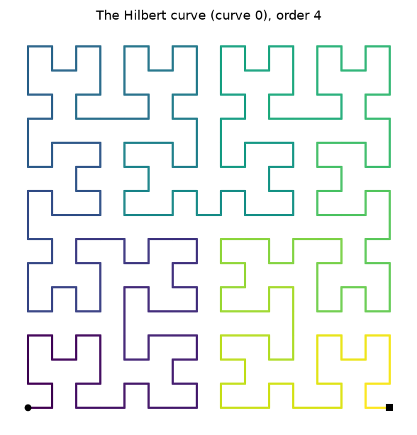
Most software knows one Hilbert curve. In fact there are forty distinct space-filling
curves of Hilbert type in two dimensions (up to rotation, reflection and reversion), as
proved by Estevez-Rams et al., "Hilbert curves in two dimensions", Rev. Cub. Fís. 34,
9 (2017). hilbertplot implements all forty with pure-numpy generation and uses them to lay
long 1-D vectors onto 2-D images.
Install
pip install "hilbertplot[plot]" # drop [plot] for a numpy-only core (no matplotlib)
Draw a curve
import hilbertplot

c = hilbertplot.curve(0)     # by index 0–39, by name ("Moore"), or by symbol
c.show(4)                    # draw order 4 in a window
pts = c.points(4)            # (256, 2) integer lattice points, in visit order
The forty curves come in named groups — hilbertplot.proper(), .improper(),
.homogeneous(), .inhomogeneous(), .generalizing() — each of which prints as a table,
and which compose:
import hilbertplot

print(hilbertplot.proper())                       # a table of the six proper curves
hilbertplot.catalog().closed().names              # ['Moore', 'Liu1', 'Improper1', 'Improper4']
hilbertplot.by_kernels(3, 5).gallery(order=3)     # draw a group as a grid of panels
In a Jupyter notebook a Curve renders itself — put hilbertplot.curve("Moore") in a cell
and you get the picture, not a repr.
One cell at a time
points(order) builds all 4**order cells. When you only need where step i lands,
encode answers in O(order) — so it works at orders no machine could materialise, and it
does so for all forty curves, not just the classic one:
import hilbertplot

c = hilbertplot.curve(0)
c.encode(5, 2)                     # (0, 3) — the cell visited at step 5, order 2
c.decode(0, 3, 2)                  # 5      — and back again
c.encode(10**18, 40)               # (751054336, 346100736) — a 2**80-cell curve
Plot data
Walk a curve and drop data[i] on the i-th cell it visits: a locality-preserving
1-D → 2-D map where nearby values stay nearby.
import numpy as np, hilbertplot

plot = hilbertplot.hilbert_plot(0, np.arange(1, 257))
plot.show("viridis")          # a matplotlib colormap name, or a list of colours to blend
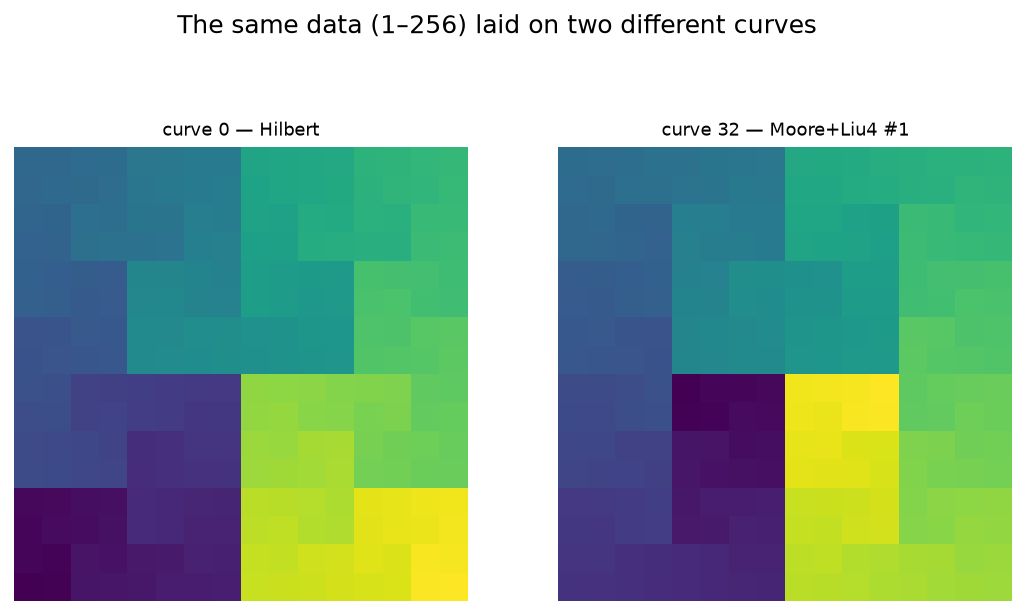
The same numbers on curve 0 and curve 32 — one reason to have all forty.
Seeing more than the data
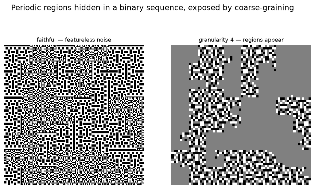
Coarse-grain it. plot.show(granularity=4) replaces each block of values by its mean.
Below, a binary sequence interleaves stretches of two periodic patterns with identical
density — invisible in the faithful plot, obvious once averaged.
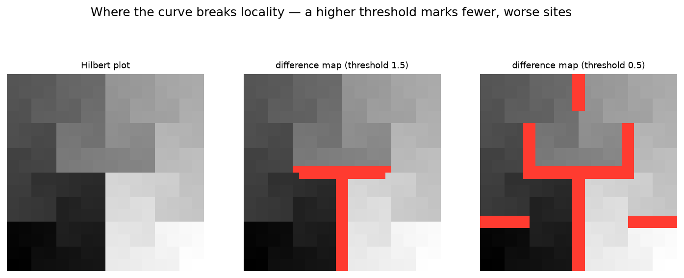
Find where locality breaks. plot.show(difference=True) marks the cells that are
neighbours in the plane but far apart along the curve. A higher threshold keeps only the
worst offenders.
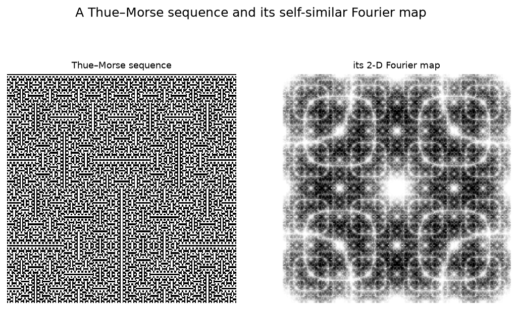
Transform it. plot.show(fourier=True) renders the 2-D Fourier map, exposing periodic
and self-similar structure — here, a Thue–Morse sequence.
Also
curve.unroll(img)— read a 2-D array back into 1-D, in curve ordercurve.grid(n)— the eightgeneralizing()curves tile anyn×nsquare, not just2ᵏcurve.label_map(order)— the grid of visit indices, as an imagecurve.difference_map(order)— where the curve breaks locality, as a fieldplot.draw(colorbar=True), ornorm=LogNorm()for heavy-tailed datahilbertplot.is_space_filling/canonical_form— check a path yourself; the same tools the test suite uses to prove all forty curves are distinct Hamiltonian pathshilbertplot.clear_cache()/cache_info()— generated curves are memoised; this frees themhilbertplot.set_cell_limit(n)— raise the guard that refuses absurdly large orders
Every figure above is reproducible: python examples/readme_figures.py. More runnable
demos are in
examples/;
the arbitrary-square classification and its impossibility proofs are in the repository's
research/quasisquares/.
License
MIT © Daniel Estevez — LICENSE
1 maintainer

Metadata
1 maintainer
Release files for hilbertplot 0.2.0
For a detailed explanation of source distributions (sdists) and built distributions (wheels), please see the package formats documentation.
Source distribution (sdist)
| File | Size | Uploaded | |
|---|---|---|---|
| hilbertplot-0.2.0.tar.gz | 72.8 kB | Details |
Built distribution (wheel)
| File | Interpreter | ABI | Platform | Reset |
|---|---|---|---|---|
| hilbertplot-0.2.0-py3-none-any.whl | Python 3 | none | any | Details |
Total release size: 127.3 kB
Release files / hilbertplot-0.2.0.tar.gz
| Download URL | hilbertplot-0.2.0.tar.gz |
|---|---|
| Size | 72.8 kB |
| Tags | Source |
|
SHA-256 checksum How to use checksums |
88aab83ff88505fd4646a10a58437f9cdbd1693c1fa02888acb1a8fdb23ac212
|
|
BLAKE2b-256 checksum How to use checksums |
b80c941958a81afbbb6d3a44453124231bf64f32f47526a75f99d9c29e359920
|
| Upload date | |
|
Uploaded using Trusted Publishing? What is trusted publishing? |
Yes |
| Uploaded via |
twine/6.1.0 CPython/3.13.14
|
Provenance
Provenance describes where a file came from. On PyPI, provenance is shared via attestations, which provide a verifiable record of the build or publishing details. View details, limitations and caveats.


PyPI Publish Attestation
PyPI verified that this artifact, at this checksum, originated from the publisher listed below.
Signed by GitHub Actions, verified by PyPI on Jul 25, 2026.
Transparency logRelease files / hilbertplot-0.2.0-py3-none-any.whl
| Download URL | hilbertplot-0.2.0-py3-none-any.whl |
|---|---|
| Size | 54.4 kB |
| Tags | Python 3 |
|
SHA-256 checksum How to use checksums |
86b2d57de03b0b56226545121d25a626888d2d2ecbea264d9181e8ee964151fc
|
|
BLAKE2b-256 checksum How to use checksums |
bb57dc82e8b030f83eb7328f65ec16acabab9f7c4566d4588f1c4acdb2087c4d
|
| Upload date | |
|
Uploaded using Trusted Publishing? What is trusted publishing? |
Yes |
| Uploaded via |
twine/6.1.0 CPython/3.13.14
|
Provenance
Provenance describes where a file came from. On PyPI, provenance is shared via attestations, which provide a verifiable record of the build or publishing details. View details, limitations and caveats.
PyPI Publish Attestation
PyPI verified that this artifact, at this checksum, originated from the publisher listed below.
Signed by GitHub Actions, verified by PyPI on Jul 25, 2026.
Transparency log













