A real-time synthetic data stream simulator based on historical data.

Project description
historical2realtime
Transform static, tabular historical data into a live, real-time synthetic data stream.
Overview
historical2realtime is a Python library designed to natively handle complex datetime features, discover fixed relationships across columns, and enforce data quality constraints automatically. By leveraging the Synthetic Data Vault (SDV) and pandas, it translates static logs and events into a live stream, fully equipped with simulated chronological pacing and real-time drift compensation.
Key Features
- Seasonality-Aware Conditional Generation: Unlike static samplers, this library enforces strict temporal conditions (Month, Day, Hour, Minute) during the synthesis process. This ensures that the generated stream respects real-world seasonal patterns, peak hours, and cyclical trends found in your historical data.
- Engine for End-to-End Pipeline Simulation: It seamlessly integrates with data-movement libraries (like Parsons) or Native connectors to stream to any destination connector (e.g., Supabase, details in Advanced Integration Example) . So its a powerful engine for testing complex data pipelines and architectural scenarios, complete with dynamically adjustable speedup factors for rapid, scaled-time testing.
- Native Datetime Handling: Automatically converts, combines, and scales temporal features, transforming static timestamps into relative minute streams, then use it train the SDV model.
- Fixed Relationship Discovery: Scans your schema to identify and preserve absolute and partial fixed relationships between the input columns "id_columns" and other columns.
- Automatic Quality Constraints: Extracts value distribution constraints and dynamically enforces them through closure-based resampling loops, to discard any numerically illogical generated rows.
- Real-Time Drift Compensation: Employs dynamic loop synchronization math that actively calculates and compensates for execution drift (mostly come from speedup process), maintaining exact chronological pacing.
- Multi-Date Chronological Integrity: Seamlessly handles datasets with multiple datetime columns (e.g., Order Time, Expected Delivery, Actual Delivery). By converting secondary dates into relative minute offsets against the primary event, the model inherently respects absolute chronological logic, mathematically preventing temporal paradoxes (like a delivery occurring before an order is placed).
- Production-Grade Async Engine: Equipped with native
asynciosupport for high-concurrency simulations. This enables realistic streaming from multiple sources simultaneously while maintaining peak resource efficiency and zero-block performance. - Replay support: You can make the library perform simulations using the same original data by setting the parameter
is_synthetic=False, while retaining the real-time flow simulation and speedup features.
Installation
pip install historical2realtime
Quick Start
from historical2realtime import simulate_realtime_stream
import logging

# # Configure basic logging for the simulator
logging.basicConfig(level=logging.INFO, format='%(asctime)s - %(message)s')

# Execute the real-time simulation orchestrator
simulate_realtime_stream(
    file_name="historical_data.csv",
    output_file_name="live_stream.csv",
    main_date_col="Event_Timestamp", # The primary datetime column used to calculate event pacing and chronological order
    id_columns=["Doc_ID", "Doc_Type"], # This is not limited to traditional 'IDs'; it includes any column where some or all values strictly dictate another column's value
    target_row_count=1000, #The total number of rows to simulate before terminating the stream.
    speedup_factor=1.0, # #1.0 is real-time rate  (the same rate of your input data)   #e.g if the real-time rate was 60s and you set factor 2.0 that means the sleeping time before generatting the new row will be 30s instead of 60s
    default_interval_seconds=60, #Fallback polling interval applied if no chronological datetime columns are present in the dataset (main_date_col= None)
    is_synthetic=True, #If True, train model and generate synthetic data. If False, replay mode simulator. Defaults to True.
)
What happens next?
Once you execute the script, simulate_realtime_stream performs the following sequence under the hood:
- Model Training: It ingests your historical data, analyzes the schema, discovers relationships, and trains a generative model (GaussianCopulaSynthesizer) to understand the distribution and temporal pacing of your dataset.
- Continuous Simulation Loop: It begins generating highly realistic synthetic rows one by one.
- Chronological Pacing: Instead of dumping all rows simultaneously, it calculates the exact time interval to the next event and physically pauses the script execution (scaled by your
speedup_factor) to simulate real-world time passing. - Live Streaming: It continuously appends each newly generated row to
live_stream.csv. This file now acts as a live, organically growing data stream that your dashboards (Excel, PowerBI, Tableau, etc.) can connect to and auto-refresh in real-time.
⚠️ WARNING: Blocking Behavior (in default mode) When
generator_mode=False, thesimulate_realtime_streamfunction start a long-running, continuous loop that utilizestime.sleep(). If used in this default mode, you must run this function in a separate process (separate python file with separate terminal). If you need integration with Connectors (databases, APIs,..etc), use the flexible modegenerator_mode=True, details in the topic of Quick Start with Generator mode.
Real-World Example: Live Hospital Cash Flow Dashboard
To see historical2realtime in action, the following screenshot is from Excel real time dashboard feed by historical2realtime engine that used to stream hospital cash flow data into a live-updating CSV file.
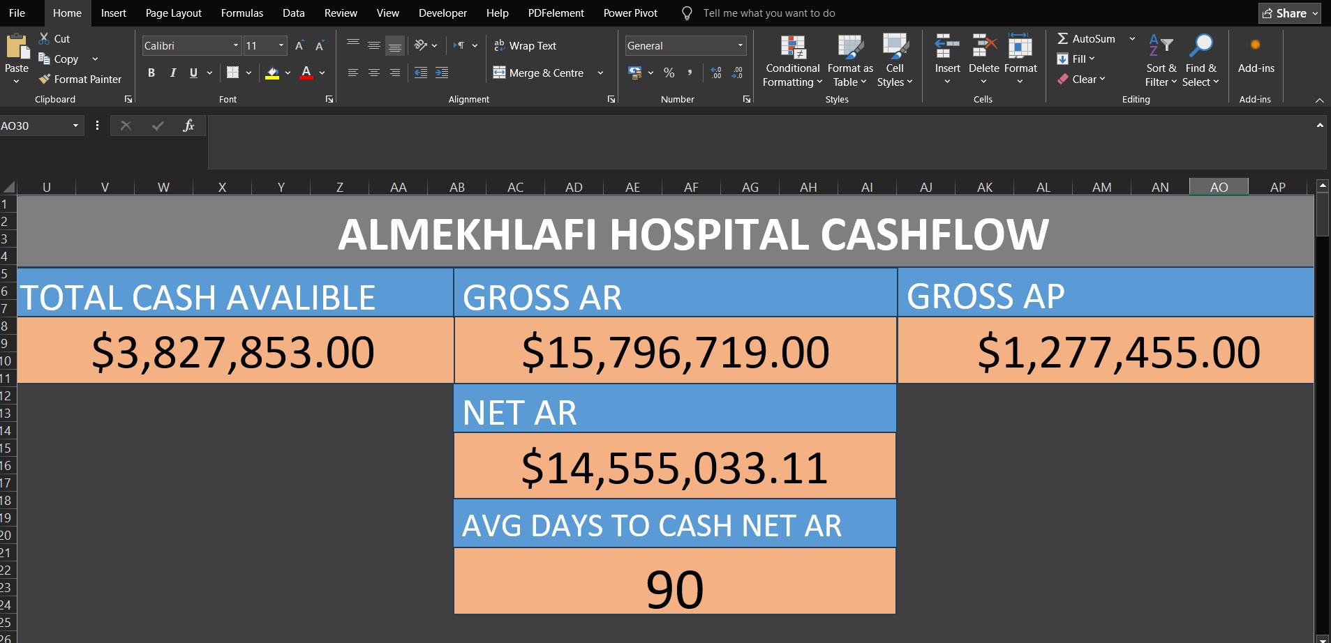
The Workflow:
- Data Streaming:
historical2realtimecontinuously simulates and writes realistic financial transactions to a local CSV file, respecting chronological constraints. - Live Connection: A Microsoft Excel workbook connects directly to this CSV using Power Query.
- Auto-Refresh: The Power Query connection is configured with a strict 1-minute auto-refresh interval.
- Real-Time Dashboarding: As Excel pulls the latest simulated data, automatically update Table and the live financial monitoring dashboard (e.g Dashboard in the above screenshot).
Hospital ERP Cashflow & Liquidity Dataset is the historical/input data that used in the above screenshot scenario and other examples.
Quick Start with Generator mode
If you want to process the generated row directly in your application (e.g., adding Calculation columns, sending them to an API...etc), you can enable generator_mode:
from historical2realtime import simulate_realtime_stream
import logging

# # Configure basic logging for the simulator
logging.basicConfig(level=logging.INFO, format='%(asctime)s - %(message)s')

# Initialize the stream as a generator
stream = simulate_realtime_stream(
	file_name="historical_data.csv",
	main_date_col="Event_Timestamp",
	id_columns=["Doc_ID", "Doc_Type"],
	target_row_count=1000,
	speedup_factor=500.0,
	generator_mode=True # Enables yielding rows instead of blocking
)

# Iterate over the generated rows in real-time
for row in stream:
    # 'row' is a pandas DataFrame containing the newly generated record
    print("New simulated row generated:", row)
    # Add your custom downstream processing logic here
What happens next?
The same Default mode Workflow but sincegenerator_mode=True It yields each row iteratively, allowing your code to capture and process the data dynamically on the fly (you are inside the generation loop and Instead of saving the new row in a csv file you have the control of the next steps).
Advanced Integration Example: Streaming to Supabase
This advanced implementation guide demonstrates how to synchronize your live synthetic stream into a Supabase (PostgreSQL) database using the Parsons library.
- Note: You can use the native PostgreSQL library or Supabase API/SDK. However, in this example, I used Parsons because it includes many connectors, and the example can be traced to establish connections with other connectors.
Step-by-Step Implementation
1. Configure Supabase Environment Variables
The Parsons library uses the Postgres connector to interact with Supabase under the hood. You need to provide your Supabase database credentials. In the synchronization script below, I set them as environment variables.
- PGHOST: Your Supabase Database Host (found in your Project > Connect > choose Direct type > choose Session pooler from Connection Methods > credentials will be in box beside Connection string).
- PGPORT: Default is
5432. - PGDATABASE: Usually
postgres. - PGUSER: Usually
postgres.your-project-id. - PGPASSWORD: Your database password.
2. Create and run stream_to_supabase Script
#install Parsons
#pip install parsons[all]

import os
from parsons import Table
from parsons.databases.postgres import Postgres
from historical2realtime import simulate_realtime_stream
import logging

# # Configure basic logging for the simulator
logging.basicConfig(level=logging.INFO, format='%(asctime)s - %(message)s')

# Setup Supabase Credentials # this is one time step and its recommand to done on terminal by command like: set VARIABLE_NAME=value
os.environ['PGHOST'] = 'host_url' #example: 'aws-0-ap-southeast-2.pooler.supabase.com'
os.environ['PGDATABASE'] = 'postgres'
os.environ['PGUSER'] = 'postgres.your-project-id'
os.environ['PGPASSWORD'] ='Your-database-password'
os.environ['PGPORT'] = '5432'

# Initialize Parsons Postgres Connector
db = Postgres()
target_table="supabase_table_name"


# Initialize the stream as a generator
stream = simulate_realtime_stream(
	file_name="historical_data.csv",
 	main_date_col="Event_Timestamp",
 	id_columns=["Doc_ID", "Doc_Type"],
	target_row_count=100,
	speedup_factor=500.0,
	generator_mode=True # Enables yielding rows instead of blocking
)

# Iterate over the generated rows in real-time
for df_row in stream:
    # 'df_row' is a pandas DataFrame containing only the newly generated record
    print("New simulated row generated...")
    # convert headers to small letters without spaces :
    df_row.columns = df_row.columns.str.lower().str.replace(" ", "_")
    # Convert  new row DataFrame into list of dict
    df_row=[df_row.iloc[0].to_dict()]
    # Convert to Parsons Table and push to Supabase #its highly recommend to create the table first (before start streaming), to avoid table schema inconsistent errors between parsons_table and supabase_table
    parsons_table = Table(df_row)
    db.copy(parsons_table, target_table, if_exists='append')
Congratulations! You now have an engine that updates your database on the cloud, and you can test the performance of your applications with near-real data equipped with speedup Feature.
API Reference
simulate_realtime_stream
The core orchestrator function that initializes the SDV model, mutates state, and yields the synthetic time-series stream.
| Parameter | Type | Description |
|---|---|---|
file_name |
str |
Path to the historical tabular data file (supports .csv, .xls, .xlsx). |
output_file_name |
str |
Path where the real-time synthesized stream will be saved and updated. |
main_date_col |
str / list / None |
The primary datetime column used to calculate event pacing and chronological order. If the date and time are split across multiple columns, provide them as a list (e.g., ['Date', 'Time']). Crucial for multi-date datasets: Always select the column representing the first chronological event (e.g., Order_Time in a logistics dataset containing Expected_Delivery and Actual_Delivery). |
id_columns |
list |
Columns acting as identifiers (Primary key and Foreign key) or having fixed logical relationships with other fields. This is not limited to traditional 'IDs'; it includes any column where some or all values acting as Foreign key (strictly dictate another column's value e.g., in the example dataset "Doc_Type" have full-fixed/partial-fixed realtionships with columns: "Entity_Name" "AI_Contract_Discount" "AI_Denial_Rate" "Status" "Cash_Impact_Direction", so you have to include "Doc_Type" in the id_columns parameter). Important: Accurately defining this list is a critical step to guarantee high-quality, logically sound output. |
target_row_count |
int |
The total number of rows to simulate before terminating the stream. |
speedup_factor |
float |
Multiplier used to divide the simulated time, increasing the stream's speed relative to real time. simulated_time=real_time/speedup_factor. 1.0 (default) |
training_sample_size |
int |
Number of historical rows to use for training the generative model.0 (default) to train the entire dataset. |
default_interval_seconds |
int |
Fallback polling interval applied if no chronological datetime columns are present in the dataset (when main_date_col=None ). 20 (default) |
generator_mode |
bool |
If True, yields an iterator (generator) for downstream processing instead of blocking execution. If False, blocks execution and writes rows directly to the output file. False (default). |
qa_attempts |
int |
The total number of QA attempts when applying the historical data constraints. |
is_synthetic |
bool |
If True, train model and generate synthetic data. If False, replay mode simulator (generate data from the original input rows as it) . True (default). |
Advanced Under-the-Hood Mechanics
For developers extending the library, understanding the internal architecture of core.py is critical:
- Dynamic State: Before passing data to the SDV synthesizer, pandas DataFrames undergo aggressive, sequential schema transformations. The pipeline actively translates main_date_col into normalized, then used to add a new column "time_to_next_event_minutes". This column represents the difference in minutes between each row and the next row in the main date column. When a new row is generated, the value in this filed is used to determine the sleep time before generating the next row (simulating real-time).
- Relative Chronological Anchoring: To eliminate temporal paradoxes in datasets with multiple date columns, the pipeline executes
convert_dates_to_relative_minutesprior to training. This mathematically transforms all secondary timestamps into numeric minute-differentials relative to themain_date_col. The SDV model trains on these numeric offsets instead of absolute dates. During real-time synthesis,restore_dates_from_relative_minutesdynamically reconstructs the exact branch timestamps, guaranteeing that subsequent events (e.g., delivery) follow the anchor event (e.g., order creation). - Fixed Relationship Discovery:
discover_fixed_relationshipsScans schema to identify and preserve absolute and partial fixed relationships between the input columns "id_columns" and other columns, then Builds a mapping dictionarylookup_dictwhich used later to correct generated synthetic data in_apply_lookup_correction. - Closure-Based Constraint Enforcement: Data quality of numeric columns is maintained through hidden scope closures. The
_enforce_quality_constraintsfunction relies on Bounding Box constrainsnum_cols_constrains. It continuously checks generated rows and iteratively resamples any row that violates the extracted percentage distribution (details in the topic Mathematical Formulation ). - Loop Synchronization Math: Real-time generation is subject to Python's inherent execution latency. To prevent lag, the final simulation loop calculates
simulated_delay_secondsusing the generated time to the next event and thespeedup_factor. It then actively calculatesspeedup_driftto dynamically adjustadjusted_now, effectively compensating for the execution time of the loop itself.
Use Case Scenarios: Who Can Benefit?
historical2realtime is designed for a variety of professional and educational contexts where static data isn't enough:
- Data Infrastructure & Pipeline Architects: Perfect for the design or optimization phase of data pipelines. It allows architects to simulate Parallel Multi-Source with high-velocity data flows to test infrastructure, verify ETL logic, and ensure system resilience before going live.
- Data Science Students & Teachers: Ideal for those learning data analysis who need to experience interacting with a "live" database environment. It provides a realistic streaming experience for practicing real-time SQL queries, data cleaning, and stream processing without waiting for real-world events to occur.
- BI & Data Analysts: A vital tool for designing monitoring dashboards (e.g., Power BI, Tableau). When real-world data updates too slowly for efficient testing, this library allows analysts to accelerate the data pace, enabling rapid debugging, error detection, and visual verification of dashboard triggers.
- Software & Backend Developers: Enables faster end-to-end application testing. Developers can verify how their applications handle incoming data streams immediately after database integration, significantly reducing the time required for integration testing and scenario validation.
- Quality Assurance (QA) & Compliance Teams: Essential for enterprises adhering to strict data privacy regulations. By masking or dropping sensitive PII (Personally Identifiable Information) from historical datasets prior to training, QA teams can leverage the library to generate a legally compliant, anonymized synthetic stream. The inherent statistical "noise" in the generated data ensures privacy while preserving business logic and edge cases for rigorous, risk-free system testing.
Important Notes & Best Practices
To get the most accurate and efficient results out of historical2realtime, read the following guidelines:
- Balancing Speed and Quality: If relationship discovery or model training is taking too long, you can accelerate the process by decreasing the
training_sample_size. However, use caution: reducing the sample size too much will significantly degrade the quality, realism, and statistical integrity of the generated data. - Capturing Seasonality: For the model to accurately capture and generate seasonal trends, time-of-day patterns, and monthly variations, it is highly recommended that your input data spans at least one full year.
- Parameter Accuracy is Critical: The integrity of your output relies heavily on accurately defining your parameters. Ensure you correctly identify your
id_columnsand carefully select the rightmain_date_col(especially when dealing with datasets that have multiple datetime columns). - Handling Calculation Columns: While the internal quality enforcement system try to ensure numeric logic and distributions, the library does not currently "detect" or maintain functional dependencies in Calculation Columns (columns derived via formulas from other columns). To ensure absolute mathematical consistency, it is highly recommended to remove these columns before passing the dataset to the library. You can easily re-calculate these derived fields downstream either in the stream loop (generator_mode) or in your data pipeline (e.g., using Power Query, DAX, or SQL transformations) once the synthetic stream is generated.
- Working with Unfamiliar Data (e.g., Kaggle): If you are working with a new/unknown dataset, you need to understand the data, Because You need to identify the ID columns, as well as columns that are not classified as unique ID columns but contain values behaving like IDs.
- Handling Concurrent Events: To prevent artificial time drift when simulating multiple events that share the exact same timestamp, you must partition your dataset by its logical source (e.g.,
Cashier_ID,Branch_ID) and execute them concurrently using parallel asynchronous streams. (details in the Parallel Simulation Example) - No Silver Bullet for All Tables/Cases: While the engine is designed to be highly adaptable, it is inherently difficult to guarantee perfect automated handling for every conceivable data shape, structure, or edge case. The model might occasionally struggle with some input tables/cases. However, remember that by utilizing the Generator Mode, you retain absolute granular control. You can always intercept each yielded row (which is a standard pandas DataFrame), apply custom fixes, enforce strict business logic, or transform specific values after it is generated but before it moves to your downstream pipeline.
The Asyncio Generator
The Async Engine is specifically designed for high-concurrency environments and cloud-native deployments. It ensures that the simulation of chronological delays (pacing) does not lead to cloud resource waste or server unresponsiveness.
Async Implementation Example
import asyncio
import logging
from historical2realtime.async_core import simulate_async_stream

# Configure basic logging for the simulator
logging.basicConfig(level=logging.INFO, format='%(asctime)s - %(message)s')

async def main():
    logger = logging.getLogger(__name__)
    logger.info("Starting the asynchronous simulator...")

    # Initialize the stream asynchronously.
    # Note: generator_mode is handled automatically by the async function, so there is no need to pass it.
    stream = simulate_async_stream(
        file_name="historical_data.csv",
        main_date_col="Event_Timestamp",
        id_columns=["Doc_ID", "Doc_Type"],
        target_row_count=100,
        speedup_factor=500.0
    )

    # Iterate over the generated rows in real-time using 'async for'
    async for row in stream:
        # 'row' is a pandas DataFrame containing the newly generated record
        print("New simulated row generated:\n", row)

        # Add your custom asynchronous downstream processing logic here


if __name__ == "__main__":
    asyncio.run(main())
Parallel Multi-Source Simulation (Supermarket Case Study)
This example demonstrates how to scale 'historical2realtime' to handle multiple data sources concurrently.
5 different cashiers of a supermarket were simulated, each streaming data from its own historical file located in a specific directory.
import asyncio
import os
import logging
from historical2realtime.async_core import simulate_async_stream

# Configure logging to distinguish between different cashier streams
logging.basicConfig(
    level=logging.INFO,
    format='%(asctime)s - [Cashier %(name)s] - %(message)s'
)


async def start_cashier_simulation(cashier_id: str, file_path: str):
    """
    Task worker to consume a specific cashier's data stream.
    """
    # Create a specialized logger for each cashier
    cashier_logger = logging.getLogger(cashier_id)

    try:
        # Initialize the async stream for this specific file
        stream = simulate_async_stream(
            file_name=file_path,
            main_date_col="Transaction_Date",
            id_columns=["Transaction_ID", "Cashier_ID"],
            target_row_count=100,  # Simulate 100 transactions per cashier
            speedup_factor=200.0
        )

        async for row in stream:
            # Process the generated transaction row
            # Here you can send data to a central database or a live dashboard
            cashier_logger.info(f"Transaction Generated: {row.to_dict(orient='records')[0]}")

    except Exception as e:
        cashier_logger.error(f"Simulation failed for {cashier_id}: {e}")


async def main():
    # Define the directory containing the historical CSV files
    data_directory = "supermarket_data"

    if not os.path.exists(data_directory):
        print(f"Error: Directory '{data_directory}' not found.")
        return

    # Collect all simulation tasks
    simulation_tasks = []

    # Iterate through files in the specific directory
    for file_name in os.listdir(data_directory):
        if file_name.endswith(".csv"):
            cashier_id = file_name.replace(".csv", "").upper()
            file_path = os.path.join(data_directory, file_name)

            # Create a task for each cashier stream
            task = start_cashier_simulation(cashier_id, file_path)
            simulation_tasks.append(task)

    if not simulation_tasks:
        print("No CSV files found for simulation.")
        return

    print(f"Starting parallel simulation for {len(simulation_tasks)} cashiers...")

    # Execute all simulation tasks concurrently
    # The Event Loop will manage context switching between streams automatically
    await asyncio.gather(*simulation_tasks)


if __name__ == "__main__":
    try:
        asyncio.run(main())
    except KeyboardInterrupt:
        print("\nSimulation stopped by user.")
Mathematical Formulation of Quality Guards
historical2realtime relies on mathematical framework to constrain the numerical columns outputs of generative models, ensuring the synthesized data adheres to historical structural boundaries.
Experts are welcome to evaluate and improve the methodology.
Problem Definition:
While SDV GaussianCopulaSynthesizer is lightweight and captures probabilistic correlations between variables, it often fails to follow business rules and structural boundaries within a single row. For instance, relational logic—such as ensuring a "Discount_Amount" never exceeds the "Price"—can be violated, leading the model to generate numerically illogical rows.
The problem is further complicated by the critical importance of maintaining the model's generalization when generating data; this means that any solution to the problem must preserve generalization.
Solution Summary:
The solution's concept is to compensate row-wise relationships by creating an intermediate table where each value represents the cell's weight relative to all cells in the same row. Then, after creating a ratio table, the highest and lowest values are taken from each column. This range now acts as an QA constraint for each column.
This achieves objectives of Excluding long-tail outliers (illogical generated row), and Maintaining the generality of the generated data.
Solution Details:
The algorithm starts by filtering historical data to get the numerical features/columns, then operates through three sequential stages:
1. Directional normalizing
The historical data rows/vectors are normalized. For each row vector $x = (x_1, x_2, ..., x_n)$, the transformation is defined as:
$$\hat{x}i = \frac{x_i}{\sum{j=1}^{n} |x_j| + \epsilon}$$
This normalizes the magnitudes relative to the entire row while preserving the mathematical sign (direction) of each component.
2. Extraction of max/main Constraints (Bounding-Box)
To bound the probability space while accounting for mixed-sign behaviors, the algorithm performs a static scan of the historical dataset to construct Bounding Boxes for each component $\hat{x}_i$ separating the components based on parity:
- Positive Domain: $$\mathcal{B}_i^+ = \left[ \min({ \hat{x}_i \mid \hat{x}_i \ge 0 }), \max({ \hat{x}_i \mid \hat{x}_i \ge 0 }) \right]$$
- Negative Domain: $$\mathcal{B}_i^- = \left[ \min({ \hat{x}_i \mid \hat{x}_i < 0 }), \max({ \hat{x}_i \mid \hat{x}_i < 0 }) \right]$$
This ensures that the bounds represent the historical spread without creating false "safe zones" spanning across the zero origin.
3. Directional Rejection Sampling
Because statistical generative models often produce long-tail outliers (illogical outliers e.g discount > price), the algorithm employs a strict filter based on Naive Rejection Sampling. For any newly synthesized sample $s$, its Directional normalizing transformation $\hat{s}$ is calculated. The sample is accepted if every component $\hat{s}_i$ satisfies its respective directional domain:
- If $\hat{s}_i \ge 0 \implies \hat{s}_i \in \mathcal{B}_i^+$
- If $\hat{s}_i < 0 \implies \hat{s}_i \in \mathcal{B}_i^-$
If any constraint is violated, the entire sample is instantly discarded and regenerated, up to a maximum limit of 100 retries.
Note on Dimensionality: Naive Rejection Sampling is highly effective for low-to-medium dimensional datasets. The 100-retry limit serves as a pragmatic threshold to maintain computational efficiency, in the future, may modify it to a dynamic value relative to the count and state of numerical columns.
After 100 attempts?: Currently, the code/algorithm take the best possible sample from the 100 attempts by choosing the Shortest Distance to the Bounding-Box, perhaps in the future may add a step to re-project the generated data into the Bounding-Box space after evaluating its effect on the quality of the generated data (against smoothing/shrinkage).
Release history Release notifications | RSS feed


Download files
Download the file for your platform. If you're not sure which to choose, learn more about installing packages.
Source Distribution
Built Distribution
Filter files by name, interpreter, ABI, and platform.
If you're not sure about the file name format, learn more about wheel file names.
Copy a direct link to the current filters
File details
Details for the file historical2realtime-0.2.0.tar.gz.
File metadata
- Download URL: historical2realtime-0.2.0.tar.gz
- Upload date:
- Size: 44.2 kB
- Tags: Source
- Uploaded using Trusted Publishing? No
- Uploaded via: twine/6.2.0 CPython/3.10.20
File hashes
| Algorithm | Hash digest | |
|---|---|---|
| SHA256 |
ad59baaa10476f1209ed19f369233e01fd2bd33d4bf6864d1c32e718629bf67e
|
|
| MD5 |
fdb6ef152026e7e68b3dc8a417e88864
|
|
| BLAKE2b-256 |
d8d3da839259eb1805d0089e48f3d8d37534418a176f907a161e197dbe82325d
|
File details
Details for the file historical2realtime-0.2.0-py3-none-any.whl.
File metadata
- Download URL: historical2realtime-0.2.0-py3-none-any.whl
- Upload date:
- Size: 25.0 kB
- Tags: Python 3
- Uploaded using Trusted Publishing? No
- Uploaded via: twine/6.2.0 CPython/3.10.20
File hashes
| Algorithm | Hash digest | |
|---|---|---|
| SHA256 |
83c79b71d6209aa124f6a2ae95249a33afd067805ea055d5ee7270252e377e89
|
|
| MD5 |
212a7a0ae04f8bbe130ff75779f64c91
|
|
| BLAKE2b-256 |
260f473f51d1f6808e8908adf031f5499cd3a66102abd5d600f5b5058aebb93d
|


