
Seeded multivariate analysis (NNMF / NNLS) of hyperspectral and multispectral microscopy data, with an interactive Qt GUI.

Project description
HS-MOSAIC




HS-MOSAIC (HyperSpectral Multivariate Optical Analysis Components) is a GUI for fast reconstruction and unmixing of hyperspectral imaging data — PCA, seeded NNMF and fixed-H NNLS, with GPU-accelerated backends and reproducible presets.
Initially built for coherent Raman scattering (CARS, SRS) and related hyperspectral and multispectral imaging workflows, but applicable to any spectral image stack that needs non-negative unmixing.
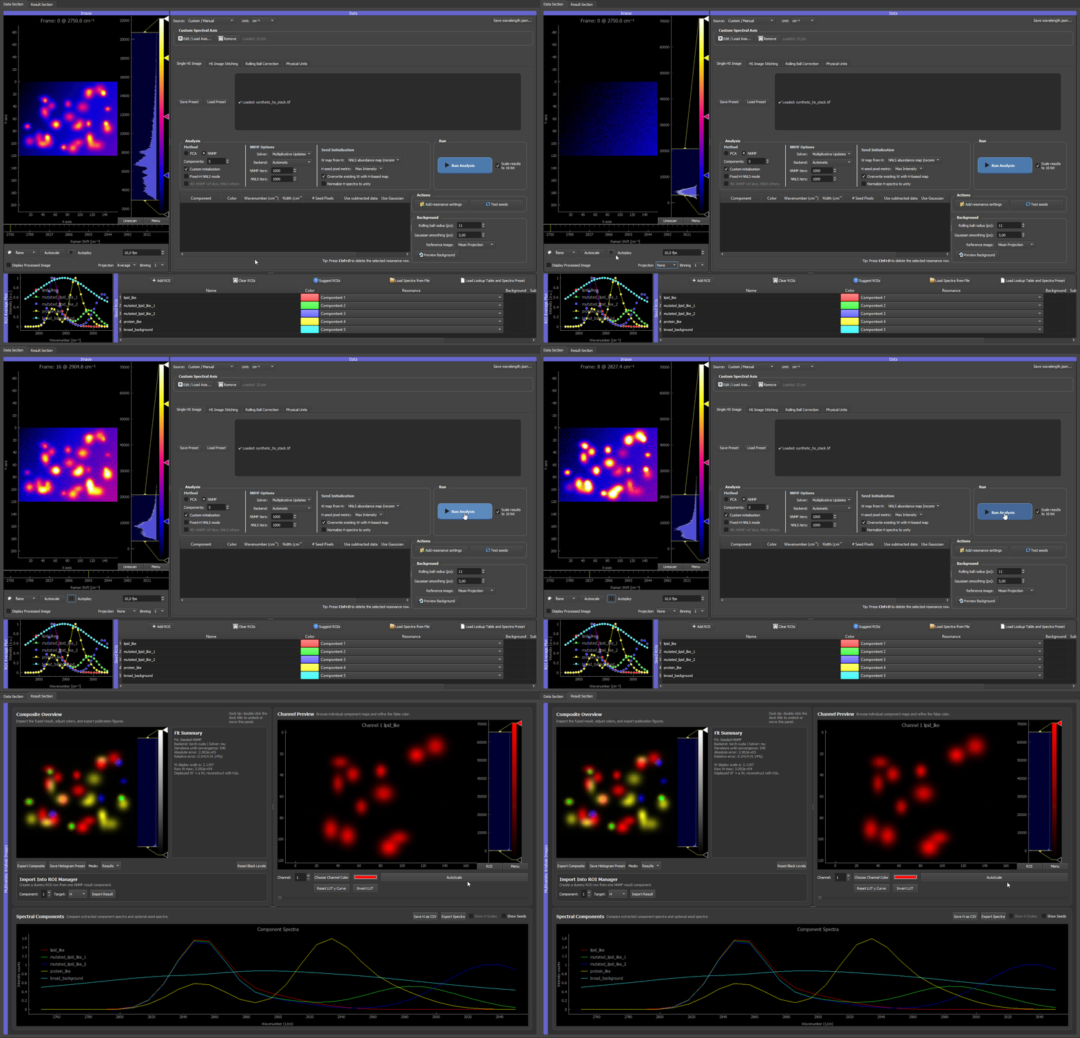
Above: a typical hyperspectral stack as it appears in HS-MOSAIC — one grayscale frame per spectral channel, with the channel slider scrolling through the cube.
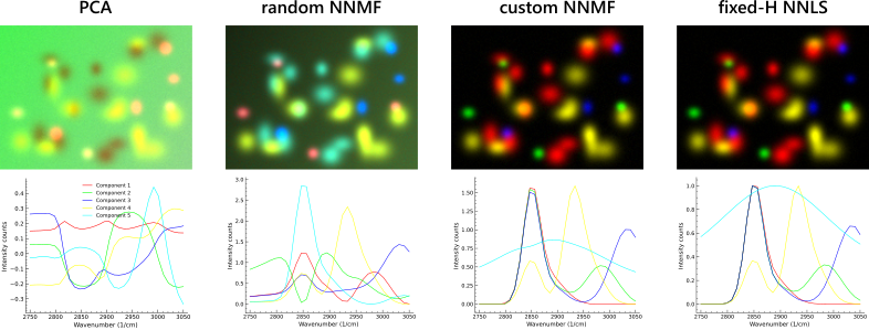
Above: the same synthetic dataset analyzed with each of the four available modes. PCA misses peaks, random NNMF mixes components, seeded NNMF and fixed-H NNLS recover the underlying blob spectra.
[!IMPORTANT] HS-MOSAIC is under active development. For published analyses, cite the exact release tag or commit hash you used so the processing workflow remains reproducible.
Why HS-MOSAIC?
- Four analysis modes in one workflow: PCA for variance-based diagnostics, random NNMF for unguided exploration, seeded NNMF for the main guided workflow, and fixed-H NNLS for spectral seed stability, particularly in 4D cross-slice / cross-time.
- Seed-first interaction: draw ROIs, load reference spectra, build Gaussian resonance models, or let the auto-suggester scan the image. Every seed source feeds the same H/W building pipeline.
- 3D and 4D stacks: per-slice or fast multislice (NNMF on a reference slice → NNLS everywhere else) for time series and z-stacks.
- Optional GPU acceleration via PyTorch with CPU fallback (scikit-learn NMF, SciPy NNLS).
- Reproducible by construction: presets save the full analysis state, ROI configuration, and seed choices. Reload the same TIFF, reload the preset, get the same result.
- Publication-friendly export: Fiji/ImageJ-compatible TIFFs, CSV spectra, LUT presets, and scale-bar metadata that survive into downstream figures.
How HS-MOSAIC unmixes a hyperspectral stack
A hyperspectral stack is a 3D cube (or 4D, with z or time): for every spatial pixel you have one full spectrum across many channels. HS-MOSAIC reorganizes that cube into a small number of components: a spatial map plus the matching spectrum that you can actually interpret as chemistry etc..
All four analysis modes operate on the same factorization: the cube is reshaped to a 2D matrix X (pixels × channels) and the algorithm looks for
X ≈ W · H
where W (pixels × components) holds the per-pixel abundance maps and H (components × channels) holds the component spectra. Each column of W is reshaped back into an image, and each row of H is plotted as a spectrum. The four modes differ only in what is held fixed and what is being learned:
| Mode | What H is |
What W is |
When to use |
|---|---|---|---|
| PCA | Variance-maximizing orthogonal directions (signed) | Pixel scores along those directions (signed) | First look at an unknown dataset; diagnostic only, not a non-negative abundance. |
| Random NNMF | Learned from data, non-negative | Learned from data, non-negative | No prior spectra exist yet; exploratory parts-based decomposition. |
| Seeded NNMF | Initialized from user ROIs / spectra, then refined | Initialized from H via NNLS / selective-score, then refined |
The main workflow. You have a rough idea of the components and want the algorithm to refine both W and H. |
| Fixed-H NNLS | Locked to the user spectra | Solved per pixel, non-negative | The spectra are trusted; only the per-pixel amounts vary. Most stable mode for 4D / cross-FOV. |
NNMF — non-negative matrix factorization
NNMF minimizes the reconstruction error under non-negativity: $$ W, H = \arg\min_{W \ge 0,; H \ge 0} \left| X - W H \right|_F^2 $$ resp.
min_{W, H ≥ 0} ‖X − W H‖_F²
Because both W and H are non-negative, the model is purely additive. There is no sign cancellation, which makes the components interpretable as physical contributions. The cost is non-convex in W and H jointly, so the initial guess (the seed) determines which local minimum the solver lands in. That is why HS-MOSAIC's seeded NNMF is the mode that actually works on hard data: the seed picks the basin of attraction.
The GUI ships two solvers: multiplicative updates (mu, default) — the classic Lee–Seung rule, optionally accelerated on GPU via PyTorch — and coordinate descent (cd) from scikit-learn, useful when MU's zero-stuck-zero property is inconvenient.
Fixed-H NNLS — non-negative least squares per pixel
Once you trust the spectra, you stop letting them drift. Fixed-H NNLS solves in pseudo code the per-pixel abundance maps W resp. for each map w given locked spectra H_seed:
for every pixel p:
    w_p  =  argmin_{w ≥ 0}  ‖x_p − w · H_seed‖²
with H_seed locked. That is the pure abundance problem: how much of each known spectrum is present in each pixel? It is the cleanest mode for 4D z- or t-stacks (every slice gets fitted against the same spectral basis) and for cross-FOV comparison.
The GUI runs NNLS through SciPy's classical Lawson–Hanson active-set solver on CPU, and through a vectorized projected-gradient + FISTA backend on PyTorch / GPU for large mosaics.
Why seeds are the scientific decision
For both seeded NNMF and fixed-H NNLS, the seed — the initial W₀ and H₀ matrices are where you encode prior knowledge: ROI-averaged spectra, imported reference spectra, Gaussian resonance models, or a W seed built from one of the H-driven modes (nnls, selective_score, h_weighted, average, empty).
[!IMPORTANT] For a reproducible run across a similar sample, the order is: pick the components, build the seeds in the ROI Manager, save a preset, then run seeded NNMF (or fixed-H NNLS if your spectra are already trusted). Reload the preset to reproduce the same result on the same data, or on a different field of view with matching components.
For the full mathematical treatment — exact convergence criteria, the MU init eps lift, scale ambiguity, the H-seed unity-scaling option, and the NNLS / FISTA convergence test see the dedicated NNMF and NNLS methods page.
Documentation
Full documentation, including tutorials and worked examples:
🌐 Live docs · 📂 docs/ in this repo
Quickest entry points:
- Quickstart — minimal end-to-end GUI workflow
- Concepts — the unmixing model and the role of seeds
- Loading data — TIFF conventions, 3D/4D axis selection, intensity handling
- Analysis modes — which mode to choose and what to expect
- Seeds, spectra, and W maps — building H and W seeds
- Presets and reproducibility — saving and restoring the full analysis state
- NNMF and NNLS methods — math, convergence criteria, references
- Workflow checklist — single-page reminder for a publication-grade run
- Troubleshooting — known issues and their fixes
To build the docs locally in a virtual environment, install the docs-requirements.txt dependencies and run the MkDocs server:
pip install -r docs-requirements.txt
mkdocs serve
At a glance
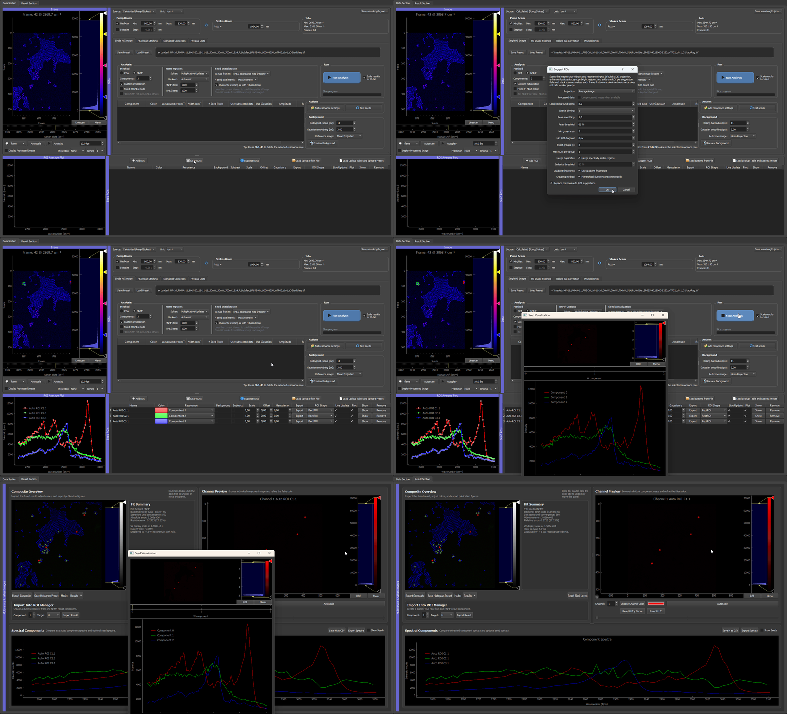
The screenshot above demonstrates the Suggest ROIs tool on the bead dataset. The same GUI handles seed building, NNMF/NNLS analysis, and result export. See docs/tutorials/03c_suggest_rois.md for the algorithm and settings reference.
Install
PyPI:
Recommended platform-independent install method. Prerequisites: A (virtual) python environment with Python ≥ 3.10 on Windows, Linux, or macOS. Optionally a supported GPU for PyTorch acceleration: NVIDIA (CUDA), Apple Silicon (MPS), Intel Arc (XPU), or AMD on Linux (ROCm).
The package is published on PyPI as hs-mosaic. Install in a virtual environment with pip.
Recommended — GPU install (the right one for your hardware):
Hyperspectral NNMF and fixed-H NNLS are heavy: typical fields of view (~10⁶ pixels × tens of channels) run in seconds on a GPU and in minutes on a CPU, with 4D z- and t-stacks multiplying the cost. Since v0.9.3 HS-MOSAIC supports three GPU backends — pick the one matching your hardware:
Open a terminal, activate your virtual python environment, and install the right torch variant for your GPU before installing hs-mosaic:
# NVIDIA CUDA GPU — install CUDA torch from PyTorch's index FIRST, then hs-mosaic.
pip install torch --index-url https://download.pytorch.org/whl/cu124
pip install hs-mosaic

# Apple Silicon (M1/M2/M3/M4) — PyPI's macOS torch wheel already includes MPS.
pip install hs-mosaic torch

# Intel Arc GPU — install XPU torch from PyTorch's index FIRST, then hs-mosaic.
pip install torch --index-url https://download.pytorch.org/whl/xpu
pip install hs-mosaic
[!IMPORTANT] PyPI does not host CUDA-enabled or XPU-enabled PyTorch wheels — only CPU torch (and CPU+MPS on macOS). For the NVIDIA and Intel variants you must install GPU-enabled torch from PyTorch's own index before
pip install hs-mosaic. The order is not optional: doing it in reverse downloads ~150 MB of CPU torch that gets immediately replaced. Apple Silicon does NOT have this issue because PyPI's macOS torch already includes MPS. This is a property of the whole Python packaging ecosystem (every GPU-accelerated package has the same constraint), not of HS-MOSAIC.
[!WARNING] Apple Silicon users: check your Python architecture before installing. If your Python is the legacy x86_64 (Intel) build running under Rosetta 2,
pip install hs-mosaic torchwill silently pintorchat the last x86_64 macOS wheel (2.2.2, NumPy-1-era) while installing NumPy 2.x alongside, producing an_ARRAY_API not founderror on launch. Run this check before installing:python -c "import platform; print(platform.machine())"
arm64= native, good to go.x86_64= Rosetta'd Intel Python — install a native arm64 Python (Miniforge or the arm64 Anaconda installer) first; the telltale path for the wrong build is/Users/<you>/opt/anaconda3/. See docs/installation.md → Apple Silicon (MPS) for the full diagnostic, the fix, and a one-linenumpy<2workaround if you can't reinstall conda right now.
For NVIDIA, pick the cu124 URL to match your CUDA driver — cu118, cu121, cu124, cu126, etc. — using the PyTorch selector.
Verify the right GPU is detected after the install:
python -c "import torch; print('CUDA:', torch.cuda.is_available()); print('MPS :', torch.backends.mps.is_available() and torch.backends.mps.is_built()); print('XPU :', hasattr(torch, 'xpu') and torch.xpu.is_available())"
Whichever line says True is the GPU backend HS-MOSAIC will use. The fit-summary backend field reports torch-cuda, torch-mps, or torch-xpu so you can confirm in the GUI.
Fallback — CPU install (no supported GPU):
For machines without a compatible GPU (e.g. AMD on Windows, ARM Linux without ROCm, CI runners, older Macs), HS-MOSAIC runs on CPU using scikit-learn's NMF and SciPy's NNLS. It works correctly but expect minutes per run instead of seconds.
pip install hs-mosaic
A
[torch]extra also exists for users who want the PyTorch FISTA-NNLS backend on CPU (sometimes faster than SciPy's per-pixel solver for very large fixed-H NNLS mosaics). It does not provide GPU acceleration on its own. See docs/installation.md for the full comparison table and for the v0.9.2 → v0.9.3[gpu]→[torch]rename recovery instructions.
From source:
Detailed installation guide and platform-specific notes: docs/installation.md.
Prerequisites — Python ≥ 3.10 on Windows, Linux, or macOS. Optionally a supported GPU for PyTorch acceleration: NVIDIA (CUDA), Apple Silicon (MPS), Intel Arc (XPU), or AMD on Linux (ROCm).
Conda (recommended) — use one of the packaged environment files in the repository root:
# Lean CPU-only environment
conda env create -f environment.yml
conda activate hs-mv-analysis

# Or: with PyTorch for the optional PyTorch NNMF/NNLS backends
conda env create -f environment-pytorch.yml
conda activate hs-mv-analysis-pytorch
Use the bundled environment.yml unless you specifically need the PyTorch-based backends. The bundled environment-pytorch.yml installs PyTorch, but it does not guarantee a CUDA-enabled build on every machine. For NVIDIA GPU acceleration, install a CUDA-enabled PyTorch build that matches your driver and platform after creating the environment from the .yml file.
pip — alternative if you prefer venv. The project is packaged; install the package itself rather than just its requirements file:
python -m venv .venv
.venv\Scripts\activate              # Windows
# source .venv/bin/activate         # Linux / macOS
pip install -e .                    # editable install from a clone
Optional extras:
pip install -e ".[torch]"           # add CPU PyTorch (NNMF MU + FISTA-NNLS backends)
pip install -e ".[dev]"             # add ruff, pytest, pyinstaller for development
For a CUDA-enabled PyTorch install, follow the official PyTorch selector after the editable install — PyPI hosts CPU-only torch wheels, so CUDA builds come from https://download.pytorch.org/whl/cu124 (or the version matching your driver). The GPU paths use the standard torch.cuda device convention; CUDA 12.6 is the recommended target when available. See GPU acceleration for the backend and platform notes, including Apple Silicon and AMD/ROCm.
Run
After a pip install (editable or from PyPI) the GUI is reachable through the hs-mosaic console entry point or as a Python module:
hs-mosaic                    # console / shortcut launcher
python -m hs_mosaic          # equivalent module form
On Windows you can also use the bundled launcher (which calls python -m hs_mosaic under the hood):
hs-mosaic.bat
A pre-built standalone Windows executable is described in docs/standalone_windows.md.
Repository layout
hs_mosaic/                          Top-level Python package (pip-installable)
├── app.py                          Application entry point — exports main()
├── __main__.py                     Enables `python -m hs_mosaic`
├── composite_image.py              Result / composite viewer
├── assets/                         Bundled icons and example metadata
└── widgets/                        Internal modules
    ├── analysis_manager.py         Analysis setup, seed handling, 4D orchestration
    ├── multivariate_analyzer.py    PCA / NNMF / NNLS core
    ├── torch_nmf.py                Optional PyTorch MU-NMF backend
    ├── nnls_pytorch.py             Optional PyTorch FISTA-NNLS backend
    ├── roi_manager_pg.py           ROI management and ROI plotting
    └── data_widgets.py             Raw-data loading and image viewer
pyproject.toml                      Package metadata, deps, hs-mosaic entry point
docs/                               User documentation (mkdocs site)
environment.yml                     Conda environment, CPU-only
environment-pytorch.yml             Conda environment, with PyTorch
requirements.txt                    pip-based dependencies (legacy; pyproject.toml is authoritative)
hs_crs_analysis_gui_cpu.spec        PyInstaller spec for standalone CPU build
hs_crs_analysis_gui_pytorch.spec    PyInstaller spec for standalone PyTorch / CUDA build
build_windows_cpu.ps1               Build script for the standalone CPU zip
build_windows_pytorch.ps1           Build script for the standalone PyTorch / CUDA zip
hs-mosaic.bat                       Windows launcher (calls `python -m hs_mosaic`)
Repository status
HS-MOSAIC is a research software project under active development. The documented workflows are intended for reproducible image analysis, but users should validate settings and outputs for their own datasets before publication.
Citation
If you use HS-MOSAIC in published work, please cite the Zenodo record and include the exact release tag or commit you used. GitHub can generate a citation from CITATION.cff.
Preliminary DOI: 10.5281/zenodo.20273076
@software{kunisch_hs_mosaic,
  author = {Kunisch, Manuel},
  title = {{HS MOSAIC} - A GUI for fast reconstruction and unmixing of hyperspectral imaging data},
  doi = {10.5281/zenodo.20273076},
  url = {https://github.com/manuel-kunisch/hs_crs_analysis_gui},
  note = {Please cite the exact release tag or commit hash used},
  year = {2026}
}
License
Copyright (C) 2026 Manuel Kunisch.
HS-MOSAIC is licensed under the GNU General Public License v3.0 or later (GPL-3.0-or-later). See LICENSE.
The source code is distributed under GPL-3.0-or-later because the application uses PyQt5, which is available under GPLv3 or a commercial Riverbank license. Documentation and project media should be cited using the software citation above unless a file states otherwise.
Acknowledgements
HS-MOSAIC builds on the scientific Python and Qt ecosystem, including NumPy, SciPy, scikit-image, scikit-learn, tifffile, matplotlib, pyqtgraph, PyQt5, QtAwesome, and optional PyTorch backends. Please also cite the method references listed in the documentation when they are relevant to your analysis.


Download files
Download the file for your platform. If you're not sure which to choose, learn more about installing packages.
Source Distribution
Built Distribution
Filter files by name, interpreter, ABI, and platform.
If you're not sure about the file name format, learn more about wheel file names.
Copy a direct link to the current filters
File details
Details for the file hs_mosaic-0.9.4.tar.gz.
File metadata
- Download URL: hs_mosaic-0.9.4.tar.gz
- Upload date:
- Size: 357.7 kB
- Tags: Source
- Uploaded using Trusted Publishing? No
- Uploaded via: twine/6.2.0 CPython/3.12.7
File hashes
| Algorithm | Hash digest | |
|---|---|---|
| SHA256 |
83f658c2d11240153c32629e67c477a557b3a306778a7746818a9a01aabbae9c
|
|
| MD5 |
b0fa86a2e2e2f8b476cd1a8feee95ee6
|
|
| BLAKE2b-256 |
e306c3d38e20755ca71b98bc6566a074e788af2e6e7763449dc45c2fbfbb4303
|
File details
Details for the file hs_mosaic-0.9.4-py3-none-any.whl.
File metadata
- Download URL: hs_mosaic-0.9.4-py3-none-any.whl
- Upload date:
- Size: 360.0 kB
- Tags: Python 3
- Uploaded using Trusted Publishing? No
- Uploaded via: twine/6.2.0 CPython/3.12.7
File hashes
| Algorithm | Hash digest | |
|---|---|---|
| SHA256 |
e391eacb57e15e9a5461fdb7f3ea6523beabfc646abb52579a1a6496e723ef76
|
|
| MD5 |
fa26d5e6e89f69d9c655c7c89950a3bb
|
|
| BLAKE2b-256 |
0aa34a7443886c8201d38a344b409d609c2da51d32c5b3ff39c0d532bf736f52
|






