A library for tree reading, embedding, and analysis of phylogenetic trees

Project description
Phylogenetic Tree Embedding
This repository provides a Python class for processing and embedding phylogenetic trees in either Euclidean or Hyperbolic geometric spaces. The class utilizes the treeswift library for handling tree structures and torch for optimizing embeddings. It offers a flexible framework for visualizing, analyzing, and embedding phylogenetic data.
📋 Requirements and Installation
To use htree, ensure your system meets the following requirements:
🖥 System Requirements
- Python Version:
>=3.12.2 - Operating System: Compatible with Linux, macOS, and Windows
📦 Dependencies
htree relies on the following Python libraries:
numpy– Numerical operationsscipy– Scientific computingmatplotlib– Visualizationtorch– PyTorch for embedding optimizationtreeswift– Phylogenetic tree processingtqdm– Progress bar for operationsimageio– Image processingimageio-ffmpeg– Video processing for animations
These dependencies will be installed automatically when you install htree via pip:
pip install htree
Tree Class
The Tree class provides an efficient way to load, process, and embed phylogenetic trees into a specified geometric space. It supports both hyperbolic and Euclidean geometries, allowing for flexible embedding choices depending on the application. The class also includes options for logging, saving intermediate states, and creating visualizations during the embedding process.
Features
- Tree Loading: Load trees from files or directly from
treeswift.Treeobjects. - Embedding: Embed trees in Euclidean or Hyperbolic spaces with customizable dimensions and parameters.
- Visualization: Generate figures or movies showing the embedding process.
- Logging: Enable detailed logging of operations for better traceability.
Initialization
The Tree class can be initialized either by providing a file path to a tree file or by directly passing a treeswift.Tree object along with a name.
from htree.tree_collections import Tree
# Initialize from file
tree = Tree("path/to/treefile.tre")
print(tree)
Tree(treefile.tre)
# Initialize from a treeswift Tree object
import treeswift as ts
t = ts.read_tree_newick("path/to/treefile.tre")
tree = Tree("treefile.tre", t)
print(tree)
Tree(treefile.tre)
Once initialized, the Tree object is ready for operations such as embedding, normalization, or visualization.
Logging Feature
The class supports logging for debugging and tracing execution. By setting logger.set_logger(True), a log file will be created in the specified directory (default: as configured in your package’s config).
import htree.logger as logger
logger.set_logger(True)
# Initialize with logging enabled
tree = Tree("path/to/treefile.tre")
print(tree)
Tree(treefile.tre)
The log will store information such as tree initialization details, embedding operations, and error messages, making it easier to trace issues or understand the workflow. Log files are named according to the current timestamp and stored in the configured log directory conf.LOG_DIRECTORY.
Methods
Once a tree is loaded, the Tree class provides functions to compute key properties like the distance matrix, diameter, and terminal node names.
distance_matrix: Computes the pairwise distance matrix between terminal nodes.diameter: Computes the diameter of the tree, defined as the longest path between any two terminal nodes.terminal_names: Returns a list of terminal node names.embed: Returns a geomtric embedding for a tree.
# Get top four terminal names
terminals = tree.terminal_names()[:4]
print(terminals)
['Diospyros_malabarica', 'Huperzia_squarrosa', 'Selaginella_moellendorffii_genome', 'Colchicum_autumnale']
# Compute their distance matrix
dist_matrix, names = tree.distance_matrix()
print(dist_matrix[:4,:4])
tensor([[0.0000, 2.0274, 2.1069, 0.9733],
        [2.0274, 0.0000, 1.7451, 1.3855],
        [2.1069, 1.7451, 0.0000, 1.4650],
        [0.9733, 1.3855, 1.4650, 0.0000]])
print(names[:4])
['Diospyros_malabarica', 'Huperzia_squarrosa', 'Selaginella_moellendorffii_genome', 'Colchicum_autumnale']
# Get tree diameter
diameter = tree.diameter()
print(diameter)
tensor(2.5342)
Tree Normalization
The normalize method scales the branch lengths of the tree such that the maximum distance (tree diameter) is set to 1. This is particularly useful before performing embeddings, to ensure consistent scaling across different trees.
# Normalize tree to have a diameter of 1
tree.normalize()
diameter = tree.diameter()
print(diameter)
tensor(1.)
Embedding in Geometric Spaces
The embed method allows embedding the phylogenetic tree into either Euclidean or hyperbolic geometry using different dimensions. This is useful for visualizing or analyzing trees in a geometric space.
geometry: The geometry type, either euclidean or hyperbolic. Defaults to hyperbolic.
dim: The dimension of the embedding space.
# Embed tree in 2D hyperbolic space
embedding = tree.embed(dim=2, geometry='hyperbolic')
print(embedding)
HyperbolicEmbedding(curvature=-15.57, model=loid, points_shape=[3, 14])
# Embed tree in 3D Euclidean space
embedding = tree.embed(dim=3, geometry='euclidean')
print(embedding)
EuclideanEmbedding(points_shape=[3, 14])
embed Method Parameters
The embed has several optional parameters (kwargs) that allow customization of the embedding process. Below is a detailed explanation of each parameter.
Parameters:
dim(int) [Required]:- Defines the number of dimensions for the embedding space. For example,
dim=2creates a 2D embedding. - Example: A 2D hyperbolic embedding is common for visualization purposes, while higher dimensions (e.g.,
dim=3) might be used for more complex analyses.
- Defines the number of dimensions for the embedding space. For example,
geometry(str) [Default:hyperbolic]:- Specifies the geometric space to use for embedding.
- Options:
hyperbolic: Embeds the tree in hyperbolic space, which is often suitable for representing hierarchical or tree-like structures.euclidean: Embeds the tree in Euclidean space, more appropriate for flat, linear structures ($$ \ell_2^2 $$ distances).
- Example:
print(tree.embed(dim=2, geometry='euclidean'))
EuclideanEmbedding(points_shape=[2, 14])
precise_opt(bool) [Default:False]:- Determines whether to use a more accurate and optimized embedding method.
- Options:
False: Quick and less computationally expensive based on spectral factorization methods.True: Provides a higher quality embedding, but may take longer due to gradient-descent optimization.
- Example:
print(tree.embed(dim=2, precise_opt=True))
HyperbolicEmbedding(curvature=-10.58, model=loid, points_shape=[3, 14])
epochs(int) [Default:1000]:- The number of epochs used for optimization during the embedding process. Relevant when
precise_opt=Trueis selected. More epochs typically yield more accurate results at the cost of increased computation time. - Example:
print(tree.embed(dim=2, precise_opt=True, epochs=2000))
HyperbolicEmbedding(curvature=-13.20, model=loid, points_shape=[3, 14])
- The number of epochs used for optimization during the embedding process. Relevant when
lr_init(float) [Default:0.01]:- The initial learning rate for the optimizer during the embedding process. This value controls how quickly the optimization process converges. A higher learning rate can speed up convergence but may overshoot optimal values, while a lower learning rate ensures a smoother, more gradual approach.
- Example:
print(tree.embed(dim=2, precise_opt=True, lr_init=0.1))
HyperbolicEmbedding(curvature=-10.58, model=loid, points_shape=[3, 14])
dist_cutoff(float) [Default:10]:- The distance cutoff used to scale the distance matrix before embedding. This helps to ensure consistent scaling across different trees, which is especially useful for comparing multiple trees embedded in the same space.
- Example:
print(tree.embed(dim=2, dist_cutoff=5.0))
HyperbolicEmbedding(curvature=-3.89, model=loid, points_shape=[3, 14])
-
save_mode(bool) [Default:False]:- Whether to save intermediate states during the embedding process. This can be useful for tracking progress or debugging, especially when using long-running optimizations with
precise_opt=True. - Example:
print(tree.embed(dim=2, precise_opt=True, save_mode=True))
HyperbolicEmbedding(curvature=-10.58, model=loid, points_shape=[3, 14])
Saved data is stored in the directory
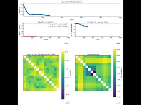
conf.OUTPUT_DIRECTORY/timestamp, wheretimestampis the current time when the embedding process starts. Each run generates a unique folder for its saved outputs. The results of the embedding process are saved in thehyperbolic_embedding_{dim}.pklfile within the timestamped folder. Whensave_mode=True, the following additional metrics are saved in the same directory during each epoch of the embedding process:- Relative Error: The normalized difference between the estimated and actual distance matrices at each epoch.
- Weights: The normalization weights used in the cost during each epoch's optimization.
- Learning Rates: The learning rate applied during the optimization process.
- Scale Booleans: Information regarding if the scale learning is enabled in each epoch.
- Whether to save intermediate states during the embedding process. This can be useful for tracking progress or debugging, especially when using long-running optimizations with
-
export_video(bool) [Default:False]:- Whether to generate a visual representation (video) of the embedding process. This can be helpful for understanding the evolution of the embedding as it progresses through optimization steps.
- Example:
tree.embed(dim=2, precise_opt=True, export_video=True)
The movie is saved in MP4 format in
confg.RESULTS_DIR/Videos/timestampwhere timestamp is the time the embedding process was initiated. In addition to the video, ifexport_video=True, individual frame images captured during the embedding process are saved inconf.OUTPUT_DIRECTORY/Images/timestamp. This allows you to view each step of the embedding visually and track its progression at a finer granularity.- Video Example: Below is a for a video demonstrating how the embedding evolves over time:
-
lr_fn(callable, optional):- Specifies a custom learning rate function for the optimization process. The function takes in arguments like the current epoch, total epochs, and a list of losses, and returns a float value representing the learning rate at that epoch. If provided, the actual learning rate is computed as the product of the initial learning rate (
lr_init) and the value returned by this function. If not provided, an adaptive learning rate is used, adjusting based on the progress of the optimization process. - Example:
def custom_learning_rate(epoch: int, total_epochs: int, loss_list: List[float]) -> float:
  """
  Calculate a dynamic learning rate based on the current epoch and total number of epochs.
  Parameters:
  - epoch (int): The current epoch in the training process.
  - total_epochs (int): The total number of epochs in the training process.
  - loss_list (list): A list of recorded loss values (can be used for further custom logic).

  Returns:
  - float: The dynamic learning rate for the current epoch.

  Raises:
  - ValueError: If `total_epochs` is less than or equal to 1.
  """

  if total_epochs <= 1:
      raise ValueError("Total epochs must be greater than 1.")

  # Example: Reduce learning rate as training progresses
  decay_factor = 0.5  # Factor by which to decay the learning rate
  loss_threshold = 0.01  # Loss threshold for further reduction
  decay_start_epoch = int(0.7 * total_epochs)  # When to start decaying

  # Reduce learning rate if the epoch is beyond a certain point
  if epoch > decay_start_epoch:
      # Learning rate decays based on the remaining epochs
      decay_rate = 1 - (epoch - decay_start_epoch) / (total_epochs - decay_start_epoch)
  else:
      decay_rate = 1.0  # No decay before the threshold
  # Further adjust learning rate if recent loss has not improved sufficiently
  if len(loss_list) > 1 and loss_list[-1] > loss_threshold:
      decay_rate *= decay_factor
  return  decay_rate
tree.embed(dim=2, precise_opt=True, lr_fn=custom_learning_rate, lr_init = 0.01)
- Specifies a custom learning rate function for the optimization process. The function takes in arguments like the current epoch, total epochs, and a list of losses, and returns a float value representing the learning rate at that epoch. If provided, the actual learning rate is computed as the product of the initial learning rate (
-
scale_fn(callable, optional): +A custom function that determines whether scale learning should occur during the optimization process. The function takes the current epoch, total epochs, and a list of losses as input, and returns a boolean value. IfTrue, scale learning is performed during that epoch; otherwise, it is skipped. If not provided, the default behavior is to enable scale learning during the early epochs of training based on a predefined ratio.- Example:
def custom_scale(epoch: int, total_epochs: int, loss_list: List[float]) -> bool:
  """
  Determine whether scale learning should occur based on the current epoch and total number of epochs.

  Parameters:
  - epoch (int): The current epoch in the training process.
  - total_epochs (int): The total number of epochs in the training process.
  - loss_list (list): A list of recorded loss values (can be used for further custom logic).

  Returns:
  - bool: `True` if scale learning should occur, `False` otherwise.

  Raises:
  - ValueError: If `total_epochs` is less than or equal to 1.
  """
  if total_epochs <= 1:
      raise ValueError("Total epochs must be greater than 1.")

  # Define the ratio of epochs during which scale learning should be applied
  curv_ratio = 0.3  # For example, learning happens during the first 30% of epochs

  return epoch < int(0.6 * total_epochs)
tree.embed(dim=2, precise_opt=True, scale_fn=custom_scale)
-
weight_exp_fn(callable, optional):- A custom function to dynamically compute the weight exponent during the optimization process. The function takes the current epoch and total epochs as input, and returns a float representing the weight exponent for that epoch. The weight exponent determines how distances are weighted during optimization. If not provided, a default behavior is applied, where weighting changes over the course of the training based on the progress of the optimization process.
- Example:
def custom_weight_exponent(epoch: int, total_epochs: int,loss_list: List[float]) -> float:
   """
   Calculate the weight exponent based on the current epoch and total number of epochs.
   Parameters:
   - epoch (int): The current epoch in the training process.
   - total_epochs (int): The total number of epochs in the training process.
   - loss_list (list): A list of recorded loss values (can be used for further custom logic).

   Returns:
   - float: The calculated weight exponent for the current epoch.

   Raises:
   - ValueError: If `total_epochs` is less than or equal to 1.
   """
   if total_epochs <= 1:
       raise ValueError("Total epochs must be greater than 1.")

   # Define a ratio that determines how long to apply no weights
   no_weight_ratio = 0.3  # Example ratio: first 30% of epochs without weighting
   no_weight_epochs = int(no_weight_ratio * total_epochs)
   # No weighting for the first part of the training
   if epoch < no_weight_epochs:
       return 0.0  # No weighting initially
   # Gradually increase the negative weight exponent after the no-weight phase
   return -(epoch - no_weight_epochs) / (total_epochs - 1 - no_weight_epochs)
tree.embed(dim=2, precise_opt=True, weight_exp_fn=custom_weight_exponent)
Saving and Copying Trees
The class provides utility functions to save and copy trees:
save(): Save the tree to a file in Newick format.
copy(): Create a deep copy of the tree object, useful for making modifications without affecting the original tree.
# Save tree to a file
tree.save("path/to/treefile2.tre")
# Copy the tree object
tree_copy = tree.copy()
MultiTree Class
The MultiTree class offers a versatile framework for managing multiple phylogenetic trees, allowing them to be loaded from various sources, processed, and embedded into geometric spaces. This class supports both hyperbolic and Euclidean embeddings, providing a flexible approach for different applications. It is subscriptable, enabling efficient selection and manipulation of tree subsets. For example, if multitree contains a collection of phylogenetic trees, an expression like multitree[:5] would return a new MultiTree instance containing only the first five trees, preserving the original structure and functionality. Additionally, the class includes logging capabilities and utility functions such as distance matrix computation and tree saving.
Features
- Flexible Tree Loading: Load trees from files, lists, or dictionaries of
Treeobjects. - Embedding Options: Jointly embed trees in hyperbolic or Euclidean spaces with customizable dimensions and optimization settings.
- Distance Matrix: Compute an aggregate distance matrix for tree comparisons, with optional confidence matrix.
- Tree Saving: Save trees in Newick format.
- Logging: Enable logging to track the operations performed on the
MultiTreeobject for debugging and traceability.
Initialization
The MultiTree class can be initialized from a variety of sources, including file paths, lists of trees of named trees, lists of trees from treeswift.
from htree.tree_collections import MultiTree
# Initialize from a Newick file
multitree = MultiTree("path/to/trees.tre")
print(multitree)
MultiTree(trees.tre, 844 trees)
# Initialize from a list of trees
import treeswift as ts
tree1 = ts.read_tree_newick("path/to/treefile1.tre")
tree2 = ts.read_tree_newick("path/to/treefile2.tre")
tree_list = [tree1, tree2]  # List of trees
multitree = MultiTree('mytrees', tree_list)
print(multitree)
MultiTree(mytrees, 2 trees)
print(multitree.trees)
[Tree(Tree_0), Tree(Tree_1)]
# Initialize from a list of named trees
from htree.tree_collections import Tree
named_trees = [Tree('a', tree1), Tree('b', tree2)]
multitree = MultiTree('mTree', named_trees)
print(multitree)
MultiTree(mTree, 2 trees)
print(multitree.trees)
[Tree(a), Tree(b)]
Once initialized, the MultiTree object provides methods for tree embedding, saving, and distance matrix computation.
Logging Feature
Enable logging for detailed tracking of actions and errors during the MultiTree operations. When enabled, logs will be written to a file with a timestamp in the filename.
# Initialize with logging enabled
import htree.logger as logger
logger.set_logger(True)
multitree = MultiTree("path/to/trees.tre")
print(multitree)
MultiTree(trees.tre, 844 trees)
Logs can be useful for debugging and provide insights into the tree loading, embedding, and saving processes.
Distance Matrix and Terminal Names
The terminal_names method in MultiTree returns the union of terminal (leaf) names from all trees, removing duplicates. The distance_matrix method computes a matrix that represents the average pairwise distances between nodes corresponding to the terminal names, using a customizable aggregation function func. For each tree, a distance matrix is first constructed for the leaf nodes in the union set of terminal names. If some terminal nodes are not present in a particular tree, the corresponding values in the matrix are replaced with NaN. The aggregation function func is then applied across these matrices to compute the final average distance matrix.
It’s important that the provided func automatically removes NaN values; otherwise, it will raise an error. Examples of valid functions include torch.nanmean (default) and torch.nanmedian, which both handle NaN values correctly. Optionally, a confidence matrix can be returned, indicating the proportion of non-NaN values for each element in the distance matrix. The method = 'fp' computes the average distance based on a weighted scheme where each tree has a weight -- equivalent to the relative similarity of it's distance matrix to the average distance matrix.
multitree = MultiTree("path/to/trees.tre")[:10]
print(multitree)
MultiTree(mTree, 10 trees)
print(multitree.trees)
[Tree(tree_1), Tree(tree_2), Tree(tree_3), Tree(tree_4), Tree(tree_5), Tree(tree_6), Tree(tree_7), Tree(tree_8), Tree(tree_9), Tree(tree_10)]
# Compute the distance matrix with default aggregation (mean)
avg_mat, conf, labels = multitree.distance_matrix()
print(avg_mat[:4,:4])
tensor([[0.0000, 0.7049, 1.2343, 0.5929],
        [0.7049, 0.0000, 1.3234, 0.6870],
        [1.2343, 1.3234, 0.0000, 1.0143],
        [0.5929, 0.6870, 1.0143, 0.0000]])
# Compute the distance matrix with custom aggregation
import torch
avg_mat, conf, labels = multitree.distance_matrix(func=torch.nanmedian)
print(avg_mat[:4,:4])
tensor([[0.0000, 0.5538, 0.9043, 0.5240],
        [0.5538, 0.0000, 1.1598, 0.5902],
        [0.9043, 1.1598, 0.0000, 0.8635],
        [0.5240, 0.5902, 0.8635, 0.0000]])
avg_mat, conf, labels = multitree.distance_matrix(method='fp')
print(avg_mat[:4,:4])
tensor([[0.0000, 0.6760, 1.1487, 0.5696],
        [0.6760, 0.0000, 1.2801, 0.6613],
        [1.1487, 1.2801, 0.0000, 0.9627],
        [0.5696, 0.6613, 0.9627, 0.0000]])
# Compute the union of all terminal names (removes duplicates)
print(multitree.terminal_names()[:4])
['Allamanda_cathartica', 'Alsophila_spinulosa', 'Amborella_trichopoda', 'Aquilegia_formosa']
Embedding Trees
The embed method in MultiTree allows you to jointly embed trees in a hyperbolic or Euclidean space, specifying the geometry, dimension, and other customizable parameters for optimization. It is flexible enough to handle both hyperbolic and Euclidean embeddings, with additional parameters like learning rate, total epochs, and scaling options. The method returns a MultiEmbedding object, which can be used for further analysis or visualization.
# Embed trees in a 2D hyperbolic space
multiemb_hyperbolic = multitree.embed(dim=2, geometry='hyperbolic')
print(multiemb_hyperbolic)
MultiEmbedding(10 embeddings)
print(multiemb_hyperbolic.embeddings)
[HyperbolicEmbedding(curvature=-0.84, model=loid, points_shape=[3, 24]), HyperbolicEmbedding(curvature=-0.84, model=loid, points_shape=[3, 76]), HyperbolicEmbedding(curvature=-0.84, model=loid, points_shape=[3, 71]), HyperbolicEmbedding(curvature=-0.84, model=loid, points_shape=[3, 70]), HyperbolicEmbedding(curvature=-0.84, model=loid, points_shape=[3, 63]), HyperbolicEmbedding(curvature=-0.84, model=loid, points_shape=[3, 80]), HyperbolicEmbedding(curvature=-0.84, model=loid, points_shape=[3, 60]), HyperbolicEmbedding(curvature=-0.84, model=loid, points_shape=[3, 76]), HyperbolicEmbedding(curvature=-0.84, model=loid, points_shape=[3, 82]), HyperbolicEmbedding(curvature=-0.84, model=loid, points_shape=[3, 51])]
# Embed trees in a 3D Euclidean space
multiemb_euclidean = multitree.embed(dim=3, geometry='euclidean')
print(multiemb_euclidean)
MultiEmbedding(10 embeddings)
print(multiemb_euclidean.embeddings)
[EuclideanEmbedding(points_shape=[3, 24]), EuclideanEmbedding(points_shape=[3, 76]), EuclideanEmbedding(points_shape=[3, 71]), EuclideanEmbedding(points_shape=[3, 70]), EuclideanEmbedding(points_shape=[3, 63]), EuclideanEmbedding(points_shape=[3, 80]), EuclideanEmbedding(points_shape=[3, 60]), EuclideanEmbedding(points_shape=[3, 76]), EuclideanEmbedding(points_shape=[3, 82]), EuclideanEmbedding(points_shape=[3, 51])]
The embed method takes several key parameters that allow for fine-tuned control of the embedding process:
dim: Specifies the number of dimensions for the embedding space (e.g., 2 for 2D or 3 for 3D).geometry: Specifies whether the embedding should be in 'hyperbolic' or 'euclidean' space.precise_opt: Controls the accuracy of the embedding process. This can be passed through kwargs or defaulted to the value inconf.ENABLE_ACCURATE_OPTIMIZATION.epochs: The number of epochs (iterations) to run the optimization for embedding. It defaults toconf.TOTAL_EPOCHSbut can be overridden.lr_init: The initial learning rate for the optimization process. It defaults toconf.LEARNING_RATE_INIT, but you can specify a custom value.dist_cutoff: The maximum diameter for scaling the embeddings. This ensures the size of the embedding is bounded and defaults toconf.MAX_RANGE.save_mode: If set to True, the embeddings will be saved automatically during the process. The default is taken fromconf.ENABLE_SAVE_MODE.lr_fn: Allows fine-tuning of the learning rate during the process. If not specified, the default learning rate (lr_init) will be used.scale_fn: Determines if scale learning should be enabled, which impacts how distances are scaled in the embedding space.weight_exp_fn: Controls how weights are adjusted during optimization, potentially affecting the impact of different nodes' distances during learning.
Refer to the Tree class for detailed explanations and further usage examples.
Saving Trees
The save method allows you to save the trees in a file (default format is Newick).
# Save trees to a Newick file
multitree.save("path/to/output.tre")
Embedding Class
The Embedding class is an abstract base class designed to represent embeddings of points in geometric spaces, either Euclidean or hyperbolic. This class primarily serves as a foundation, and specific geometric implementations (e.g., Euclidean and Hyperbolic) are used in practice. The Embedding class supports both NumPy arrays and PyTorch tensors for point representation and can log operations if logging is enabled.
Attributes
- geometry (str): The geometry of the space, either
euclideanorhyperbolic. Default ishyperbolic. - points (torch.Tensor): A PyTorch tensor representing the points in the embedding space.
- labels (list): A list of labels corresponding to the points in the space.
Initialization
def __init__(geometry='hyperbolic', points=None, labels=None)
Parameters
- geometry (
str): The geometry type (euclideanorhyperbolic). Default ishyperbolic. - points (
Optional[Union[np.ndarray, torch.Tensor]]): Points to embed, provided as a NumPy array or PyTorch tensor. Default isNone. - labels (
Optional[List[Union[str, int]]]): Labels for the points. Default isNone.
Methods
save(filename: str)-> None: Saves the current instance of theEmbeddingclass to a file using pickle,filenameis the path where the embedding will be saved.copy() -> Embedding: Creates a deep copy of theEmbeddingobject.load(filename: str) -> Embedding: Loads anEmbeddinginstance from a file using pickle,filenameis the path from where the embedding will be loaded.
In practice, the Embedding class itself is not directly instantiated. Instead, specific subclasses like EuclideanEmbedding and HyperbolicEmbedding are utilized for the actual geometric embeddings. These subclasses extend the base Embedding class, ensuring the correct handling of points and dimensions according to the geometry in use.
Examples
from htree.embedding import Embedding
import numpy as np
# Create an embedding with hyperbolic geometry (norm requirements are not applied)
n_points = 10
dimension = 2
embedding = Embedding(geometry='hyperbolic', points=np.random.randn(dimension,n_points))
print(embedding)
Embedding(geometry=hyperbolic, points_shape=[2, 10])
# Update points
embedding.points = np.random.randn(2,150)
raise NotImplementedError("update_dimensions must be implemented by a subclass")
# Set labels
labels = [str(i) for i in range(n_points)]
embedding.labels = list(range(n_points))
# Save the embedding
embedding.save('embedding.pkl')
# Load the embedding
loaded_embedding = Embedding.load('embedding.pkl')
print(loaded_embedding)
Embedding(geometry=hyperbolic, points_shape=[2, 10])
import torch
import htree.logger as logger
logger.set_logger(True)
embedding = Embedding(geometry='euclidean', points = np.random.randn(dimension,n_points))
print(embedding)
Embedding(geometry=euclidean, points_shape=[2, 10])
EuclideanEmbedding Class
EuclideanEmbedding is a subclass of Embedding that represents an embedding in Euclidean space. It provides additional functionality specific to Euclidean geometry, such as translation, rotation, and computation of distance matrices.
Attributes
- curvature (
float): The curvature of the Euclidean space, which is always0. - geometry (
str): The geometry of the space, which is alwayseuclidean. - points (
torch.Tensor): A PyTorch tensor representing the points in Euclidean space. - labels (
List[Union[str, int]]): A list of labels corresponding to the points in the space.
Methods
translate: Translates the points by a given vector in Euclidean space.rotate: Rotates the points by a given rotation matrix in Euclidean space.center: Centers the points by subtracting the centroid from each point.centroid: Computes and returns the centroid of the points.distance_matrix: Computes and returns the distance matrix for points in Euclidean geometry.
translate Method
The translate method shifts all points in Euclidean space by a specified vector. This method ensures that the points are translated correctly by a vector of matching dimensionality. If the vector’s dimension doesn’t align with the space, it raises an error. The following example demonstrates the translation of points representing the vertices of a regular pentagon.
import matplotlib.pyplot as plt
from htree.embedding import EuclideanEmbedding
import numpy as np
# Function to generate points at the vertices of a regular pentagon
def generate_pentagon_vertices():
     angles = np.linspace(0, 2 * np.pi, 6)[:-1]  # 5 angles for 5 vertices, excluding the last one to avoid duplication
     x = np.cos(angles)
     y = np.sin(angles)
     return np.vstack((x, y))
# Function to plot points with edges, and axes
def plot_pentagon(ax, points, title, color, marker, label_text):
     ax.scatter(points[0, :], points[1, :], c=color, s=100, edgecolors='black', marker=marker, label=label_text)
     # Draw edges between consecutive points
     for i in range(points.shape[1]):
         start = i
         end = (i + 1) % points.shape[1]
         ax.plot([points[0, start], points[0, end]], [points[1, start], points[1, end]], color=color)
     # Draw the axes
     ax.axhline(0, color='black', linewidth=0.5)
     ax.axvline(0, color='black', linewidth=0.5)
     ax.set_title(title)
     ax.set_xlabel('X-axis')
     ax.set_ylabel('Y-axis')
     ax.set_aspect('equal', adjustable='box')
     ax.legend()
# Define pentagon vertices
points = generate_pentagon_vertices()
dimension = points.shape[0]
n_points = points.shape[1]
# Initialize embedding
embedding = EuclideanEmbedding(points=points)
# Create a figure for the translation
fig1, ax1 = plt.subplots(figsize=(8, 8))
# Plot the original pentagon vertices with edges
plot_pentagon(ax1, embedding.points, "Translation of Pentagon Vertices", color='black', marker='o', label_text='Original Points')
# Translate the points
translation_vector = np.random.randn(dimension)/2  # 2D translation vector
embedding.translate(translation_vector)
# Plot the translated pentagon vertices with edges
plot_pentagon(ax1, embedding.points, "Translation of Pentagon Vertices", color='green', marker='^', label_text='Translated Points')
# Show the plot for translation
plt.show()
In this example, a regular pentagon is translated by a randomly generated 2D vector, and the changes in the points are visualized on a plot.
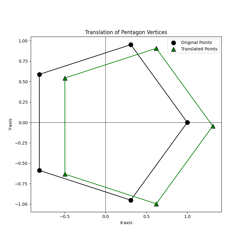
This demonstrates the effect of the translate method on the pentagon's vertices, illustrating how the points move to their new positions.
rotate Method
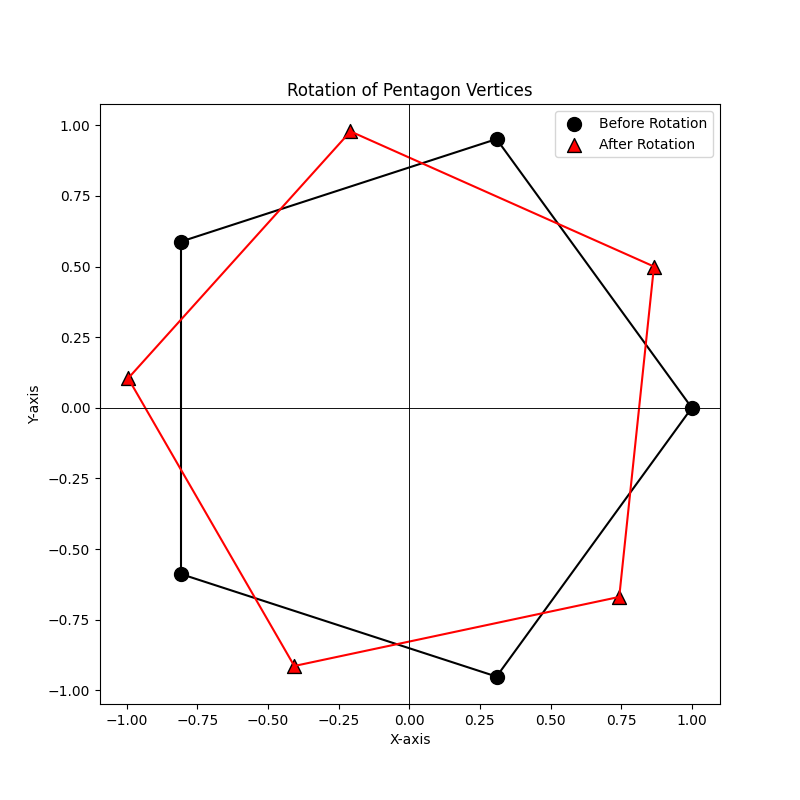
The rotate method allows you to rotate the points in Euclidean space by applying a rotation matrix. The method automatically handles the conversion of NumPy arrays to PyTorch tensors, checks for the validity of the rotation matrix, and ensures that the points are rotated correctly. In this example, we create a set of points (the vertices of a pentagon), rotate them by 30 degrees using a rotation matrix, and plot the points before and after rotation.
embedding = EuclideanEmbedding(points=points, labels=labels)
# Create a figure for the rotation
fig2, ax2 = plt.subplots(figsize=(8, 8))
# Plot the translated pentagon vertices with edges and labels before rotation
plot_pentagon(ax2, embedding.points, "Rotation of Pentagon Vertices", color='black', marker='o', label_text='Before Rotation')
# Convert degrees to radians and define the 2x2 rotation matrix
theta = np.radians(30)
rotation_matrix = np.array([
    [np.cos(theta), -np.sin(theta)],
    [np.sin(theta), np.cos(theta)]
])
# Rotate the points
embedding.rotate(rotation_matrix)
# Plot the pentagon vertices with edges after rotation
plot_pentagon(ax2, embedding.points, "Rotation of Pentagon Vertices", color='red', marker='^', label_text='After Rotation')
# Show the plot for rotation
plt.show()
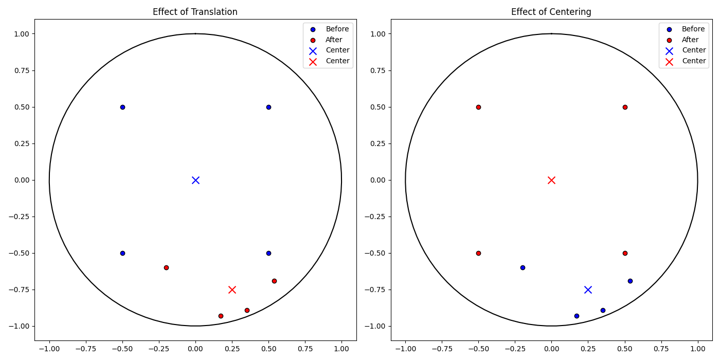
center,centroid, and distance_matrix Methods
The center method centers the points in Euclidean space by subtracting the centroid from each point. This operation shifts the points so that their centroid becomes the origin. The centroid method computes the geometric center of the points in Euclidean space by calculating the mean of each dimension.
# updating points
new_points = torch.tensor([[1.0, 2.0, 3.0], [4.0, 5.0, 6.0]])
embedding.points = new_points  # This will automatically update dimensions and other attributes.
print(embedding.points)
tensor([[1., 2., 3.],
        [4., 5., 6.]], dtype=torch.float64)
print(embedding.centroid())
tensor([2., 5.], dtype=torch.float64)
embedding.center()
print(embedding.points)
tensor([[-1.,  0.,  1.],
        [-1.,  0.,  1.]], dtype=torch.float64)
print(embedding.centroid())
tensor([0., 0.], dtype=torch.float64)
The distance_matrix method computes the pairwise Euclidean distances between all points in the embedding. This results in a symmetric matrix where each element at position (i, j) represents the distance between point i and point j.
distance_matrix,labels = embedding.distance_matrix()
print(distance_matrix)
tensor([[0.0000, 1.4142, 2.8284],
        [1.4142, 0.0000, 1.4142],
        [2.8284, 1.4142, 0.0000]], dtype=torch.float64)
HyperbolicEmbedding Class
This HyperbolicEmbedding class is designed to represent embeddings in hyperbolic space, supporting both the Poincare and Loid models. While the class provides an infrastructure for hyperbolic embeddings, it's primarily intended to be extended through subclasses that specifically handle the Poincare and Loid models.
Purpose
The key purpose of this class is to allow switching between these two models (PoincareEmbedding and LoidEmbedding), which are different ways to represent points in hyperbolic space. However, we do not directly use this class in practice. Instead, we rely on its subclasses, which tailor the functionality specifically for Poincare or Loid embeddings.
Key Features
- Curvature Scaling: The curvature of the hyperbolic space can be adjusted, but this does not affect the constraint that hyperbolic points must always have unit norms. The curvature merely scales distances between points.
- Model Switching: The
switch_modelmethod allows converting between Poincare and Loid embeddings seamlessly. - Distance Calculations: Methods like
poincare_distancecompute distances in the Poincare model, while transformation methods (to_poincareandto_loid) switch between representations.
This structure ensures flexibility in working with hyperbolic embeddings, particularly when needing to switch between models while maintaining consistent point norms.
Attributes
- curvature (
torch.Tensor): The curvature of the hyperbolic space, which must always be negative (e.g., -1). It scales distances between points but does not affect the requirement that points in hyperbolic space must have a unit norm.. - model (
str): Specifies whether the Poincare or Loid model is used to represent the points. Default ispoincare, but you can switch toloid. - points (
torch.Tensor or np.ndarray): Contains the points in the hyperbolic space, represented as either NumPy arrays or PyTorch tensors. - labels (
List[Union[str, int]]): A list of labels corresponding to the points in the space.
Methods
- s
witch_model: Switches between the Poincare and Loid models. If the current model is Poincare, it switches to Loid, and vice versa. poincare_distance(x, y): Computes the Poincare distance between two pointsxandyin the Poincare model.to_poincare(vectors): Transforms vectors from the Loid model to the Poincare model.to_loid(vectors): Transforms vectors from the Poincare model to the Loid model.
PoincareEmbedding Class
The PoincareEmbedding class represents a hyperbolic embedding space using the Poincare model. It extends from the HyperbolicEmbedding class and introduces additional features specific to the Poincare geometry.
Constructor and Attributes
def __init__(self, curvature: Optional[float] = -1, points: Optional[Union[np.ndarray, torch.Tensor]] = None, labels: Optional[List[Union[str, int]]] = None) -> None
- curvature (
float): The curvature of the hyperbolic space (default is-1). - points (
torch.Tensor): Points in the Poincare space. - labels (
List[Union[str, int]]): Optional labels for the points.
The constructor initializes the embedding in Poincare space and checks the point norms to ensure they adhere to the Poincare constraints.
Methods
_norm2: Computes and returns the squared L2 norm of the points in the embedding. This is useful for validating that points remain within the appropriate norms for the Poincare model.distance_matrix: Computes the pairwise distance matrix between the points using the Poincare distance formula.centroid: Computes the centroid of the points in the Poincare embedding. It supports two modes:default: Uses the Loid model for initial calculations (based on the definition in On Procrustes Analysis in Hyperbolic Space), then projects the centroid back to Poincare space.Frechet: Uses a gradient-based optimization method (Frechet Mean) to find the centroid by minimizing the sum of squared distances.
translate: Translates the points by a given vector, while ensuring that the resulting points still comply with the norm constraints of the Poincare model.rotate: Rotates the points by a given rotation matrix. The method ensures that the matrix is a valid rotation matrix and adjusts it if necessary.center: Centers the points by translating them to the centroid calculated by thecentroidmethod.
Example: Initialization
This example illustrates the initialization and manipulation of a hyperbolic embedding using the PoincareEmbedding class. A set of points is first generated with a specified dimensionality and associated labels. The embedding is created in hyperbolic space with the default curvature of -1. The process includes computing norms of the embedded points and updating the points themselves, which automatically adjusts the embedding's dimensionality and size. The use of tensors allows for seamless updates to the point set, maintaining the consistency of the embedding's properties.
from htree.embedding import PoincareEmbedding
import numpy as np
# Number of points to embed and their dimensionality
n_points = 10
dimension = 3
# Create labels for each point (as strings)
labels = [str(i) for i in range(1,n_points+1)]
# Generate random points with a small variance
points = np.random.randn(dimension,n_points)/10
# Initialize the Poincare embedding with the generated points and labels
embedding = PoincareEmbedding(points = points, labels = labels)
print(embedding)
HyperbolicEmbedding(curvature=-1.00, model=poincare, points_shape=[3, 10])
# Change the curvature of the embedding to -2
embedding.curvature = -2
print(embedding)
HyperbolicEmbedding(curvature=-2.00, model=poincare, points_shape=[3, 10])
# Get the dimensionality of the embedding (which is 3 for now)
print(embedding.dimension)
3
# Get the number of points in the embedding (10 points)
print(embedding.n_points)
10
import torch
# Create a new set of points using a tensor (2-dimensional points, 4 total points)
new_points = torch.tensor([[-0.5, 0.5, 0.5, -0.5], [-0.5, 0.5, -0.5, 0.5]])
# Update the embedding points with the new tensor
embedding.points = new_points
# Check the new dimensionality (should be 2 after updating points)
print(embedding.dimension)
2
# Check the new number of points (should be 4 after updating points)
print(embedding.n_points)
4
Example: Using distance_matrix, centroid, and switch_model
This section demonstrates the functionality of key methods in the PoincareEmbedding or HyperbolicSpace class, focusing on distance calculations, centering the embedding, computing the centroid, switching models, and converting to the Loid model.
# Compute the distance matrix between all points in the embedding
print(embedding.distance_matrix()[0])
tensor([[0.0000, 2.4929, 2.0416, 2.0416],
        [2.4929, 0.0000, 2.0416, 2.0416],
        [2.0416, 2.0416, 0.0000, 2.4929],
        [2.0416, 2.0416, 2.4929, 0.0000]], dtype=torch.float64)
# Change the curvature of the embedding to -0.5 and observe how the distance matrix changes
# Distances scale with 1 / sqrt(-curvature), so as curvature becomes shallower (closer to 0), distances increase.
embedding.curvature = -0.5
print(embedding.distance_matrix()[0])
tensor([[0.0000, 4.9858, 4.0832, 4.0832],  # Distances increase due to the scaling effect of the curvature
        [4.9858, 0.0000, 4.0832, 4.0832],
        [4.0832, 4.0832, 0.0000, 4.9858],
        [4.0832, 4.0832, 4.9858, 0.0000]], dtype=torch.float64)
# Compute the centroid of the points in the embedding (default mode)
print(embedding.centroid())
tensor([[0.],  # The centroid lies at the origin in this case
        [0.]], dtype=torch.float64)
# Compute the centroid using the Frechet mode, which applies a different calculation
print(embedding.centroid(mode = 'Frechet'))
tensor([[0.],
        [0.]], dtype=torch.float64)
# Switch the model from Poincare to Loid, transforming the points accordingly
loid_embedding = embedding.switch_model()
print(loid_embedding)
HyperbolicEmbedding(curvature=-0.50, model=loid, points_shape=[3, 4])  # Model switched to 'loid'
Example: Using translate, rotate, and center
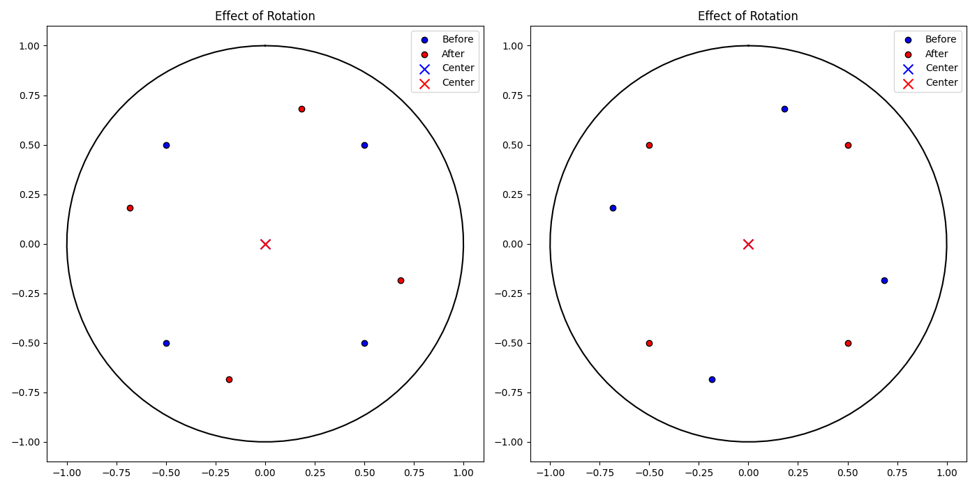
This section demonstrates the functionality of key methods in the PoincareEmbedding or HyperbolicSpace class, focusing on distance calculations, translating and rotating the embedding, as well as the centering.
# Function to plot embeddings before and after a transformation
def plot_embedding_comparison(points_before, points_after, center_before, center_after, title, ax):
    # Plot Poincaré unit circle (domain) in black
    theta = np.linspace(0, 2 * np.pi, 100)
    circle_x = np.sin(theta)
    circle_y = np.cos(theta)
    ax.plot(circle_x, circle_y, 'k-')
    ax.scatter(points_before[0, :], points_before[1, :], color='blue', label='Before', edgecolor='k')
    ax.scatter(points_after[0, :], points_after[1, :], color='red', label='After', edgecolor='k')
    ax.scatter(center_before[0], center_before[1], color='blue', marker='x', s=100, label='Center')
    ax.scatter(center_after[0], center_after[1], color='red', marker='x', s=100, label='Center')
    ax.set_title(title)
    ax.set_aspect('equal')
    ax.legend()
# Get the current points from the embedding
points = embedding.points
# Compute the centroid of the embedding before any transformation
center = embedding.centroid()
# Get the current points from the embedding
points = embedding.points
# # Compute the centroid of the embedding before any transformation
center = embedding.centroid()
# Define a translation vector to shift the embedding points
translation_vector = np.array([0.25, -0.75])
embedding.translate(translation_vector)
# The embedding now has updated points, reflecting the translation
HyperbolicEmbedding(curvature=-0.5, model=poincare, points_shape=[2, 4])
# Translation is a distance-preserving map, so distances between points should remain consistent
print(embedding.distance_matrix())
tensor([[0.0000, 4.9858, 4.0832, 4.0832],
        [4.9858, 0.0000, 4.0832, 4.0832],
        [4.0832, 4.0832, 0.0000, 4.9858],
        [4.0832, 4.0832, 4.9858, 0.0000]], dtype=torch.float64)
fig, axs = plt.subplots(1, 2, figsize=(14, 7))
# Plot the effect of translation on the embedding
plot_embedding_comparison(points, embedding.points, center, embedding.centroid(), 'Effect of Translation', axs[0])
# Get the updated points after translation
points = embedding.points
center = embedding.centroid()
# Return the centroid of the embedding (affected by the translation)
print(embedding.centroid())
tensor([[ 0.2500],
        [-0.7500]], dtype=torch.float64)
# Move the points to their centroid
embedding.center()
# Plot for centering operations
plot_embedding_comparison(points, embedding.points, center, embedding.centroid(), 'Effect of Centering', axs[1])
plt.tight_layout()
plt.show()
fig, axs = plt.subplots(1, 2, figsize=(14, 7))
# Store the initial points of the embedding
points_before = embedding.points
# Compute the centroid of the embedding
center = embedding.centroid()
# Define a rotation angle of 30 degrees (converted to radians)
theta = np.radians(30)
# Create the 2D rotation matrix for the given angle
rotation_matrix = np.array([[np.cos(theta), -np.sin(theta)],
                            [np.sin(theta), np.cos(theta)]])
# Rotate the points in the embedding using the rotation matrix
embedding.rotate(rotation_matrix)
# Plot the original vs rotated points for the first subplot
plot_embedding_comparison(points_before, embedding.points, center, embedding.centroid(), 'Effect of Rotation', axs[0])
# Store the points after the first rotation
points_before = embedding.points
# Compute the centroid again (after rotation)
center = embedding.centroid()
# Define a rotation angle of -30 degrees (to rotate in the opposite direction)
theta = np.radians(-30)
# Create the 2D rotation matrix for the opposite rotation
rotation_matrix = np.array([[np.cos(theta), -np.sin(theta)],
                            [np.sin(theta), np.cos(theta)]])
# Apply the second rotation (rotating back)
embedding.rotate(rotation_matrix)
# Plot the second rotation for the second subplot
plot_embedding_comparison(points_before, embedding.points, center, embedding.centroid(), 'Effect of Rotation', axs[1])
plt.tight_layout()
plt.show()
LoidEmbedding Class
LoidEmbedding is a class that represents the Loid model in hyperbolic space. It is derived from the HyperbolicEmbedding class and provides methods to handle points in the Loid model.
Constructor and Attributes
def __init__(self,curvature: Optional[float] = -1, points: Optional[Union[np.ndarray, torch.Tensor]] = None, labels: Optional[List[Union[str, int]]] = None) -> None
- curvature (
float): The curvature of the hyperbolic space (default is-1). - points (
torch.Tensor): Points in the Loid space. - labels (
List[Union[str, int]]): Optional labels for the points.
Methods
_norm2: Computes and returns the Lorentzian norm (squared) of the points in the embedding. This is useful for validating that points remain within the appropriate norms for the Loid model.distance_matrix: Computes the distance matrix for the points in the Loid model, returning a tensor of shape(n_points, n_points).centroid: Computes the centroid of the points in the Loid space. Supports different modes (default,Frechet).translate: Translates the points by a given vector in the Loid model. Ensures the vector follows the norm constraints of the model.rotate: Rotates the points by a given matrixR. Raises aValueErrorifRis not a valid rotation matrix.center: Centers the points by translating them to the centroid calculated by thecentroidmethod.
Example: Initialization
This example demonstrates the initialization and manipulation of a hyperbolic embedding using the LoidEmbedding class. Points are generated with a specified dimensionality and associated labels, and the embedding is created in hyperbolic space with a default curvature of -1. Norms are computed to add an extra dimension, adjusting the points and embedding accordingly. Tensor operations ensure efficient updates to the point set, preserving the embedding’s properties.
from htree.embedding import LoidEmbedding
import numpy as np
# Number of points to embed and their dimensionality
n_points = 10
dimension = 3
# Create labels for each point (as strings)
labels = [str(i) for i in range(1,n_points+1)]
# Generate random points with a small variance
points = np.random.randn(dimension, n_points)
# Add the extra dimension: sqrt(1 + norm(points)**2)
norm_points = np.linalg.norm(points, axis=0)
points = np.vstack([np.sqrt(1 + norm_points**2), points])
# Initialize the Loid embedding with the updated points and labels
embedding = LoidEmbedding(points=points, labels=labels)
HyperbolicEmbedding(curvature=-1.00, model=loid, points_shape=[4, 10])
# Change the curvature of the embedding to -2
embedding.curvature = -2
print(embedding)
HyperbolicEmbedding(curvature=-2.00, model=loid, points_shape=[4, 10])
# Get the Lorentzian norm (squared) of the embedding
print(embedding._norm2())
tensor([-1.0000, -1.0000, -1.0000, -1.0000, -1.0000, -1.0000, -1.0000, -1.0000,
        -1.0000, -1.0000], dtype=torch.float64)
# Get the dimensionality of the embedding (which is 3 for now)
print(embedding.dimension)
3
# Get the number of points in the embedding (10 points)
print(embedding.n_points)
10
import torch
# Create a new set of points using a tensor (2-dimensional points, 4 total points)
new_points = np.array([[-0.5, 0.5, 0.5, -0.5], [-0.5, 0.5, -0.5, 0.5]])
norm_points = np.linalg.norm(new_points, axis=0)
new_points = np.vstack([np.sqrt(1 + norm_points**2), new_points])
# Update the embedding points with the new tensor
embedding.points = new_points
# Check the new dimensionality (should be 2 after updating points)
print(embedding.dimension)
2
# Check the new number of points (should be 4 after updating points)
print(embedding.n_points)
4
Example: Using distance_matrix, centroid, and switch_model
This example demonstrates the creation and manipulation of a hyperbolic embedding using the LoidEmbedding class. Points are generated with a specified dimensionality, and an additional dimension is added based on the Lorentzian norm (squared) of the points. The embedding is initialized in hyperbolic space with a default curvature of -1. The curvature, Lorentzian norm, dimensionality, and number of points can be queried or updated, and tensor operations ensure seamless updates to the embedding.
# Compute the distance matrix between all points in the embedding
print(embedding.distance_matrix()[0])
tensor([[0.0000, 0.9312, 0.6805, 0.6805],
        [0.9312, 0.0000, 0.6805, 0.6805],
        [0.6805, 0.6805, 0.0000, 0.9312],
        [0.6805, 0.6805, 0.9312, 0.0000]], dtype=torch.float64)
# Change the curvature of the embedding to -0.5 and observe how the distance matrix changes
# Distances scale with 1 / sqrt(-curvature), so as curvature becomes shallower (closer to 0), distances increase.
embedding.curvature = -0.5
print(embedding.distance_matrix()[0])
tensor([[0.0000, 1.8625, 1.3611, 1.3611],
        [1.8625, 0.0000, 1.3611, 1.3611],
        [1.3611, 1.3611, 0.0000, 1.8625],
        [1.3611, 1.3611, 1.8625, 0.0000]], dtype=torch.float64)
# Compute the centroid of the points in the embedding (default mode)
print(embedding.centroid())
tensor([[1.],
        [0.],
        [0.]], dtype=torch.float64)# The centroid lies at the origin in this case
# Compute the centroid using the Frechet mode, which applies a different calculation
print(embedding.centroid(mode = 'Frechet'))
tensor([[1.],
        [0.],
        [0.]], dtype=torch.float64)
# Switch the model from Loid to Poincare, transforming the points accordingly
poincare_embedding = embedding.switch_model()
print(poincare_embedding)
HyperbolicEmbedding(curvature=-0.50, model=poincare, points_shape=[2, 4])
print(poincare_embedding.distance_matrix()[0])
tensor([[0.0000, 1.8625, 1.3611, 1.3611],
        [1.8625, 0.0000, 1.3611, 1.3611],
        [1.3611, 1.3611, 0.0000, 1.8625],
        [1.3611, 1.3611, 1.8625, 0.0000]], dtype=torch.float64)
Example: Using translate, rotate, and center
This section demonstrates the functionality of key methods in the LoidEmbedding or HyperbolicSpace class, focusing on distance calculations, translating and rotating the embedding, as well as the centering.
import matplotlib.pyplot as plt
from mpl_toolkits.mplot3d import Axes3D
fig = plt.figure()
ax = fig.add_subplot(111, projection='3d')
# Function to plot embeddings before and after a transformation
def plot_hyperbolic_sheet_with_points(points, color='red', label='Scatter Points', max_radius=2):
    if isinstance(points, torch.Tensor):
        points = points.numpy()
    # Extract x, y, z from points where z = sqrt(1 + x^2 + y^2)
    x_points = points[2,:]  # z from original points as x
    y_points = points[1,:]  # y remains as y
    z_points = np.sqrt(1 + x_points**2 + y_points**2)  # Compute z based on x and y
    def hyperbolic_z(x, y):
        return np.sqrt(1 + x**2 + y**2)
    theta_vals = np.linspace(0, 2 * np.pi, 100)  # Angular coordinate
    r_vals = np.linspace(0, max_radius, 50)  # Radial coordinate
    # Convert polar to cartesian coordinates for a circular grid
    theta_grid, r_grid = np.meshgrid(theta_vals, r_vals)
    x_grid = r_grid * np.cos(theta_grid)
    y_grid = r_grid * np.sin(theta_grid)
    z_grid = hyperbolic_z(x_grid, y_grid)
    ax.plot_wireframe(x_grid, y_grid, z_grid, color='lightblue', alpha=0.5, linewidth=0.5)
    ax.scatter(x_points, y_points, z_points, color=color, s=100, label=label)
    ax.set_xticks([])  # Remove x-axis ticks
    ax.set_yticks([])  # Remove y-axis ticks
    ax.set_zticks([])  # Remove z-axis ticks
    ax.xaxis.pane.fill = False
    ax.yaxis.pane.fill = False
    ax.zaxis.pane.fill = False
    ax.xaxis.line.set_color((0.5, 0.5, 0.5))  # Light gray axis lines
    ax.yaxis.line.set_color((0.5, 0.5, 0.5))
    ax.zaxis.line.set_color((0.5, 0.5, 0.5))
    ax.set_xlabel('X axis')
    ax.set_ylabel('Y axis')
    ax.set_zlabel('Z axis')
    ax.set_title('Hyperbolic Sheet with Scatter Points')
    ax.legend()
print(embedding.centroid())
tensor([[1.],
        [0.],
        [0.]], dtype=torch.float64)
plot_hyperbolic_sheet_with_points(embedding.points, color='red', label='Points', max_radius=2.5)
translation_vector = np.random.randn(2,1)/2  # 2D translation vector
norm_point = np.linalg.norm(translation_vector, axis=0)
translation_vector = np.vstack([np.sqrt(1 + norm_point**2), translation_vector])
print(translation_vector)
[[1.26644363]
 [0.56049116]
 [0.53826492]]
embedding.translate(translation_vector)
print(embedding.centroid())
tensor([[1.2664],
        [0.5605],
        [0.5383]], dtype=torch.float64)
plot_hyperbolic_sheet_with_points(embedding.points, color='blue', label='After Tranlation', max_radius=2.5)
embedding.center()
plot_embedding_comparison(points, embedding.points, center, embedding.centroid(), 'Effect of Translation', axs[0])
# Get the updated points after translation
print(embedding.centroid())
tensor([[ 1.0000e+00],
        [-5.6656e-17],
        [-6.7987e-17]], dtype=torch.float64)
plt.show()
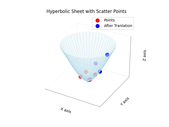
theta = np.radians(30)
rotation_matrix = np.array([ [np.cos(theta), -np.sin(theta)], [np.sin(theta), np.cos(theta)]])
# Proper Lorentzian Rotation Matrix
R = np.zeros((3,3))
R[0,0] = 1
R[1:,1:] = rotation_matrix
plot_hyperbolic_sheet_with_points(embedding.points, color='red', label='Points', max_radius=1.5)
embedding.rotate(R)
plot_hyperbolic_sheet_with_points(embedding.points, color='blue', label='After Rotation', max_radius=1.5)
plt.show()
EuclideanProcrustes Class
The EuclideanProcrustes class performs Euclidean orthogonal Procrustes analysis, which is a method used to align one embedding (source) to another embedding (target) by finding the best-fitting orthogonal transformation (rotation and translation). This process minimizes the alignment error between the two embeddings, making them as similar as possible in Euclidean space.
Constructor and Attributes
EuclideanProcrustes(source_embedding: 'Embedding', target_embedding: 'Embedding')
The constructor initializes the class with the source and target embeddings, preparing it for alignment.
- source_embedding (
Embedding): The source embedding to map from.. - target_embedding (
Embedding): The target embedding to map to.
Methods
map(embedding: 'Embedding') -> 'Embedding': This method applies the computed transformation matrix to the provided embedding (which should resemble thesource_embedding) and returns the aligned embedding. The transformation minimizes the distance between corresponding points in the source and target embeddings.
Example: Initialization
This example shows how to initialize the EuclideanProcrustes class and use it to align two embeddings. A source embedding is created, and the target embedding is generated by applying a known transformation (translation and rotation) to the source. The Procrustes method is then used to recover this transformation.
from htree.procrustes import EuclideanProcrustes
from htree.embedding import EuclideanEmbedding
import numpy as np
n_points = 10
dimension = 2
points = np.random.randn(dimension, n_points)
embedding = EuclideanEmbedding(points=points)
# Make a copy of the embedding to serve as the source embedding
source_embedding = embedding.copy()
print(source_embedding.points)
tensor([[-1.6209, -0.2308, -0.6212,  0.6591, -0.9084, -1.0451, -0.5635, -1.5712,
         -1.3372,  0.3394],
        [ 1.7770, -0.1018,  1.2887,  0.5590, -0.4241,  0.8596, -0.3132,  1.9741,
         -0.7349, -0.1978]], dtype=torch.float64)
# Create the target embedding by transforming the source embedding
target_embedding = embedding.copy()
# Apply transformation: translation + rotation
translation_vector = np.random.randn(dimension)
target_embedding.translate(translation_vector)
# Convert degrees to radians and define the 2x2 rotation matrix
theta = np.radians(30)
rotation_matrix = np.array([[np.cos(theta), -np.sin(theta)],[np.sin(theta), np.cos(theta)]])
target_embedding.rotate(rotation_matrix)
print(target_embedding.points)
tensor([[-2.1462, -0.0029, -1.0362,  0.4374, -0.4286, -1.1888, -0.1853, -2.2017,
         -0.6445,  0.5389],
        [ 1.8580,  0.9259,  1.9349,  1.9431,  0.3079,  1.3513,  0.5765,  2.0535,
         -0.1756,  1.1279]], dtype=torch.float64)
# Initialize the Procrustes model with the source and target embeddings
model = EuclideanProcrustes(source_embedding, target_embedding)
# Use the model to align the source embedding to the target
source_aligned = model.map(source_embedding)
# The aligned source embedding should now closely match the target
print(source_aligned.points)
tensor([[-2.1462, -0.0029, -1.0362,  0.4374, -0.4286, -1.1888, -0.1853, -2.2017,
         -0.6445,  0.5389],
        [ 1.8580,  0.9259,  1.9349,  1.9431,  0.3079,  1.3513,  0.5765,  2.0535,
         -0.1756,  1.1279]], dtype=torch.float64)
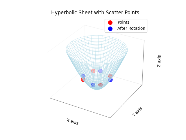
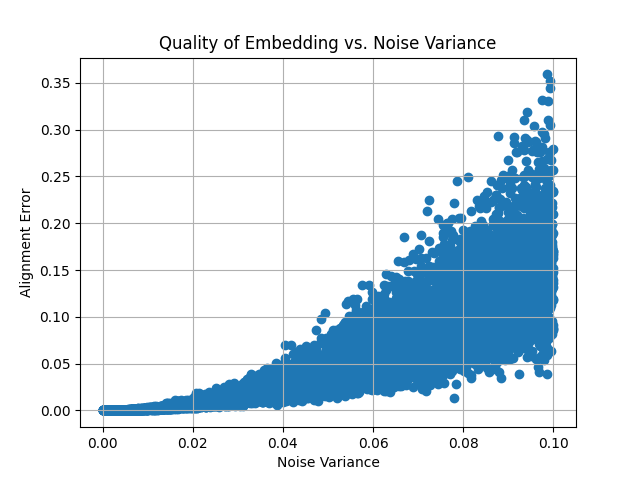
Example: Evaluating Procrustes Alignment with Noisy Embeddings
This example demonstrates the effect of adding Gaussian noise to the target embedding and evaluating the alignment quality (measured by alignment error) as noise increases. A plot is generated to visualize how the noise impacts the alignment.
import matplotlib.pyplot as plt
# Define noise variances
noise_variances = np.linspace(0, .1, 10000)  # Variances from 0 to 1
alignment_errors = []
# Loop through different noise variances
for noise_variance in noise_variances:
    noisy_target_embedding = target_embedding.copy()
    # Add Gaussian noise to the points with specified variance
    noise = np.random.normal(0, np.sqrt(noise_variance), size=noisy_target_embedding.points.shape)
    noisy_target_embedding.points += noise
    # Apply Procrustes alignment
    model = EuclideanProcrustes(source_embedding, noisy_target_embedding)
    source_aligned = model.map(source_embedding)
    # Compute alignment error (e.g., mean squared error between aligned and target points)
    alignment_error = np.mean(np.linalg.norm(source_aligned.points - noisy_target_embedding.points, axis=0))
    alignment_errors.append(alignment_error)
# Plot quality of embedding vs. noise variance
plt.scatter(noise_variances, alignment_errors, marker='o')
plt.xlabel('Noise Variance')
plt.ylabel('Alignment Error')
plt.title('Quality of Embedding vs. Noise Variance')
plt.grid(True)
plt.show()
This plot demonstrates how the alignment error increases as more noise is added to the target embedding, showing the robustness of the Procrustes analysis under varying levels of distortion.
HyperbolicProcrustes Class
The HyperbolicProcrustes class implements Hyperbolic orthogonal Procrustes analysis, which aligns one embedding (source) to another (target) through a transformation that minimizes the distance between corresponding points. This technique is particularly beneficial for aligning embeddings within hyperbolic space.
Attributes
- source_embedding (
Embedding): An instance of the source embedding from which points are mapped. - target_embedding (
Embedding): An instance of the target embedding to which points are mapped. - precise_opt (
bool): If it is set toTrue, the model creates a more accurate mapping. - logger (
logging.Logger): A logger for recording activities and events within the class, if logging is enabled.
Constructor
HyperbolicProcrustes(source_embedding: 'Embedding', target_embedding: 'Embedding', precise_opt: bool = False)
Example: Initialization
The following example illustrates how to initialize the HyperbolicProcrustes class with source and target embeddings, along with enabling logging during the initialization process.
from htree.procrustes import HyperbolicProcrustes
from htree.embedding import PoincareEmbedding
import numpy as np
n_points = 10
dimension = 2
# Generate random points for the source embedding
points = np.random.randn(dimension, n_points)/10
# Initialize the source embedding
source_embedding = PoincareEmbedding(points=points)
print(source_embedding.points)
tensor([[ 0.2135, -0.0119,  0.0454, -0.1136,  0.0334, -0.0786, -0.0686, -0.1149,
         -0.0842,  0.1199],
        [-0.0798,  0.0566,  0.1365,  0.0822, -0.0354, -0.1948, -0.1846,  0.0131,
         -0.0577,  0.0051]], dtype=torch.float64)
# Create a target embedding by copying and transforming the source
target_embedding = source_embedding.copy()
translation_vector = np.random.randn(dimension)/4
target_embedding.translate(translation_vector)
theta = np.radians(27.5)
rotation_matrix = np.array([[np.cos(theta), -np.sin(theta)],[np.sin(theta), np.cos(theta)]])
target_embedding.rotate(rotation_matrix)
print(target_embedding.points)
tensor([[-0.4023, -0.5559, -0.5553, -0.6032, -0.5126, -0.5377, -0.5346, -0.5871,
         -0.5603, -0.4777],
        [-0.4450, -0.4259, -0.3731, -0.4428, -0.4570, -0.5466, -0.5412, -0.4689,
         -0.4906, -0.4155]], dtype=torch.float64)
# Initialize the Procrustes model with the source and target embeddings
import htree.logger as logger
logger.set_logger(True)
model = HyperbolicProcrustes(source_embedding, target_embedding)
# Map the source embedding to the target space
source_aligned = model.map(source_embedding)
print(source_aligned.points)
tensor([[-0.4023, -0.5559, -0.5553, -0.6032, -0.5126, -0.5377, -0.5346, -0.5871,
         -0.5603, -0.4777],
        [-0.4450, -0.4259, -0.3731, -0.4428, -0.4570, -0.5466, -0.5412, -0.4689,
         -0.4906, -0.4155]], dtype=torch.float64)
# Switch the model of the source embedding
source_embedding  = source_embedding.switch_model()
print(source_embedding)
HyperbolicEmbedding(curvature=-1.00, model=loid, points_shape=[3, 10])
print(source_embedding.points)
tensor([[ 1.1096,  1.0067,  1.0423,  1.0401,  1.0047,  1.0923,  1.0807,  1.0271,
          1.0211,  1.0292],
        [ 0.4503, -0.0240,  0.0926, -0.2318,  0.0669, -0.1645, -0.1427, -0.2330,
         -0.1702,  0.2433],
        [-0.1684,  0.1135,  0.2788,  0.1676, -0.0709, -0.4075, -0.3840,  0.0266,
         -0.1167,  0.0103]], dtype=torch.float64)
source_aligned = model.map(source_embedding)
print(source_aligned.points)
tensor([[-0.4023, -0.5559, -0.5553, -0.6032, -0.5126, -0.5377, -0.5346, -0.5871,
         -0.5603, -0.4777],
        [-0.4450, -0.4259, -0.3731, -0.4428, -0.4570, -0.5466, -0.5412, -0.4689,
         -0.4906, -0.4155]], dtype=torch.float64)
In this example, we demonstrate the process of creating and transforming embeddings, initializing the HyperbolicProcrustes model, and aligning the source embedding to the target embedding. The logging feature can assist in monitoring the internal processes during the mapping.
Example: Evaluating Procrustes Alignment with Noisy Embeddings
We now demonstrates the effect of adding Gaussian noise to the target embedding (in Poincare domain) and evaluating the alignment quality as noise increases.
import matplotlib.pyplot as plt
# Define a trivial function to compute the alignment cost
def compute_alignment_cost(src_embedding, trg_embedding):
    cost = sum((torch.norm(src_embedding.points[:, n]- trg_embedding.points[:, n]))**2 for n in range(src_embedding.n_points))
    return cost
# Define noise variances
noise_variances = np.linspace(0, .1, 1000)  # Variances from 0 to 1
alignment_errors = []
# Loop through different noise variances
for noise_variance in noise_variances:
    noisy_target_embedding = target_embedding.copy()
    noisy_target_embedding.switch_model()
    # Add Gaussian noise to the points with specified variance
    noise = np.random.normal(0, np.sqrt(noise_variance)/2, size=noisy_target_embedding.points.shape)
    noisy_target_embedding.points += noise
    noisy_target_embedding.switch_model()
    # Apply Procrustes alignment
    model = HyperbolicProcrustes(source_embedding, noisy_target_embedding, precise_opt=False)
    source_aligned = model.map(source_embedding)
    alignment_error = np.mean(np.linalg.norm(source_aligned.points - noisy_target_embedding.points, axis=0))
    alignment_errors.append(alignment_error)
# Plot quality of embedding vs. noise variance
plt.scatter(noise_variances, alignment_errors, marker='o')
plt.xlabel('Noise Variance')
plt.ylabel('Alignment Error')
plt.title('Quality of Embedding vs. Noise Variance')
plt.grid(True)
plt.show()
This plot demonstrates how the alignment error increases as more noise is added to the target embedding, showing the robustness of the Procrustes analysis under varying levels of distortion.
MultiEmbedding Class
The MultiEmbedding class is designed to manage and align multiple embeddings in a unified framework. It provides functionality for adding, discarding, aligning, and computing aggregated distance matrices across multiple embeddings. It also supports logging for tracking progress and debugging.
Constructor and Attributes
def __init__(self)
Methods
append(embedding: 'Embedding'): Adds an embedding to the end of the collection.align(agg_func = torch.nanmean, mode = 'accurate'): Aligns all embeddings by adjusting them to a reference embedding computed by averaging their distance matrices.precise_opt: Seeembedmethod in classTree.epochs: Seeembedmethod in classTree.lr_init: Seeembedmethod in classTree.dist_cutoff: Seeembedmethod in classTree.save_mode: Seeembedmethod in classTree.scale_fn: Seeembedmethod in classTree.lr_fn: Seeembedmethod in classTree.weight_exp_fn: Seeembedmethod in classTree.func: A function to compute the aggregate distance matrix (default istorch.nanmean).
distance_matrix(func: Callable[[torch.Tensor], torch.Tensor] = torch.nanmean): Computes the aggregated distance matrix from all embeddings, replacing any missing values with estimates.reference_embedding(func: Callable[[torch.Tensor], torch.Tensor] = torch.nanmean, **kwargs): Generates a reference embedding based on the average (using functionfunc) distance matrix of all embeddings. For other variables, refer toembedmethod in classTree`.
Example: Initialization
The following example demonstrates how to initialize the MultiEmbedding class, add embeddings, and compute the aggregated distance matrix.
from htree.embedding import MultiEmbedding
from htree.embedding import EuclideanEmbedding
import numpy as np
import torch
# Initialize a MultiEmbedding object
multi_embedding = MultiEmbedding()
# Create and add multiple embeddings
n_points = 10
dimension = 2
labels = [str(i) for i in range(n_points)]
points = np.random.randn(dimension,n_points)/10
embedding1 = EuclideanEmbedding(points = points, labels = labels)
print(embedding1)
EuclideanEmbedding(points_shape=[2, 10])
multi_embedding.append(embedding1)
# Add another embedding with different dimensions
labels = [str(i) for i in range(14)]
points = np.random.randn(4,14)/10
embedding2 = EuclideanEmbedding(points = points, labels = labels)
print(embedding2)
EuclideanEmbedding(points_shape=[4, 14])
multi_embedding.append(embedding2)
labels = [str(i) for i in range(5)]
points = np.random.randn(3,5)/10
embedding3 = EuclideanEmbedding(points = points, labels = labels)
print(embedding3)
EuclideanEmbedding(points_shape=[3, 5])
multi_embedding.append(embedding3)
labels = [str(i) for i in range(7)]
points = np.random.randn(4,7)/10
embedding4 = EuclideanEmbedding(points = points, labels = labels)
print(embedding4)
EuclideanEmbedding(points_shape=[4, 7])
multi_embedding.append(embedding4)
print(multi_embedding)
MultiEmbedding(4 embeddings)
# Check the embeddings dictionary
print(multi_embedding.embeddings)
[EuclideanEmbedding(points_shape=[2, 10]),EuclideanEmbedding(points_shape=[4, 14]), EuclideanEmbedding(points_shape=[3, 5]), EuclideanEmbedding(points_shape=[4, 7])]
# another way of initialization the multiembedding
multi_embedding = MultiEmbedding()
multi_embedding.embeddings = [embedding1, embedding2, embedding3, embedding4]
print(multi_embedding.embeddings)
[EuclideanEmbedding(points_shape=[2, 10]), EuclideanEmbedding(points_shape=[4, 14]), EuclideanEmbedding(points_shape=[3, 5]), EuclideanEmbedding(points_shape=[4, 7])]
# computing the aggregate distance matrix over the union of labels
print(multi_embedding.distance_matrix()[0].shape)
torch.Size([14, 14])
# Compute the aggregated distance matrix
print(multi_embedding.distance_matrix()[0][:4,:4]) # defualt aggregation method is mean
tensor([[0.0000, 0.2846, 0.3471, 0.2391],
        [0.2846, 0.0000, 0.4289, 0.2696],
        [0.3471, 0.4289, 0.0000, 0.2342],
        [0.2391, 0.2696, 0.2342, 0.0000]], dtype=torch.float64)
# Using a different aggregation function (e.g., torch.nanmedian)
print(multi_embedding.distance_matrix(func = torch.nanmedian)[0][:4,:4])
tensor([[0.0000, 0.2747, 0.3471, 0.2391],
        [0.2747, 0.0000, 0.4289, 0.2696],
        [0.3471, 0.4289, 0.0000, 0.2342],
        [0.2391, 0.2696, 0.2342, 0.0000]], dtype=torch.float64)
Example: Reference Embedding
This section demonstrates how to compute a reference embedding using the MultiTree class and the MultiEmbedding class. The example illustrates how to load trees from Newick files, create embeddings for these trees, and calculate a reference embedding based on the average distance matrix across all embeddings.
# Load trees from Newick files
from htree.tree_collections import MultiTree
import treeswift as ts
tree1 = ts.read_tree_newick('path/to/treefile1.tre')
tree2 = ts.read_tree_newick('path/to/treefile2.tre')
# Create a MultiTree object
multitree = MultiTree('name', [tree1, tree2])
print(multitree)
MultiTree(name, 2 trees)
# Print the first 4x4 section of the average distance matrix from the trees
print(multitree.distance_matrix()[0][:4,:4])
tensor([[0.0000, 2.2280, 1.6060, 0.9966],
        [2.2280, 0.0000, 2.5171, 1.8496],
        [1.6060, 2.5171, 0.0000, 2.0671],
        [0.9966, 1.8496, 2.0671, 0.0000]])
# Create joint embeddings for the trees in 2-dimensional hyperbolic space
multiembedding = multitree.embed(dim = 2)
print(multiembedding)
MultiEmbedding(2 embeddings)
# View the embeddings for each tree
print(multiembedding.embeddings)
[HyperbolicEmbedding(curvature=-8.92, model=loid, points_shape=[3, 30]), HyperbolicEmbedding(curvature=-8.92, model=loid, points_shape=[3, 14])]
# Show the first 4x4 section of the distance matrix from the embeddings
print(multiembedding.distance_matrix()[0][:4,:4]) # hyperbolic distances are used to approxiate tree distances
tensor([[5.9791e-08, 2.1971e+00, 2.9019e-01, 6.6652e-02],
        [2.1971e+00, 1.3717e-08, 2.4854e+00, 1.2870e+00],
        [2.9019e-01, 2.4854e+00, 0.0000e+00, 1.4410e+00],
        [6.6652e-02, 1.2870e+00, 1.4410e+00, 0.0000e+00]], dtype=torch.float64)
reference = multiembedding.reference_embedding() # compute the reference point set by embedding the average distance matrix
print(reference)
HyperbolicEmbedding(curvature=-8.92, model=loid, points_shape=[3, 40])
print( reference.distance_matrix()[0][:4,:4]) # Show the distance matrix of the reference embedding
tensor([[0.0000, 2.0969, 3.1035, 1.4822],
        [2.0969, 0.0000, 2.3563, 1.9331],
        [3.1035, 2.3563, 0.0000, 3.1467],
        [1.4822, 1.9331, 3.1467, 0.0000]], dtype=torch.float64)
reference = multiembedding.reference_embedding(precise_opt=True) # Compute a more accurate reference embedding
print(reference)
HyperbolicEmbedding(curvature=-8.92, model=loid, points_shape=[3, 40])
print( reference.distance_matrix()[0][:4,:4]) # Show the more accurate distance matrix of the reference embedding
tensor([[0.0000e+00, 1.5942e+00, 2.6063e+00, 4.3736e-01],
        [1.5942e+00, 0.0000e+00, 2.1983e+00, 1.5878e+00],
        [2.6063e+00, 2.1983e+00, 0.0000e+00, 2.4947e+00],
        [4.3736e-01, 1.5878e+00, 2.4947e+00, 7.9983e-08]], dtype=torch.float64)
multiembedding = multitree.embed(dimension = 2, precise_opt=True) # Recompute embeddings in hyperbolic space with more accuracy
print(multiembedding)
MultiEmbedding(2 embeddings)
print(multiembedding.embeddings) # View the embeddings with updated curvature
[HyperbolicEmbedding(curvature=-8.30, model=loid, points_shape=[3, 30]), HyperbolicEmbedding(curvature=-8.30, model=loid, points_shape=[3, 14])]
# embedding trees in euclidean space
multiembedding = multitree.embed(dim = 2, geometry = 'euclidean')
print(multiembedding.embeddings)
[EuclideanEmbedding(points_shape=[2, 30]), EuclideanEmbedding(points_shape=[2, 14])]
print((multiembedding.distance_matrix()[0][:4,:4])**2) # Compute the squared Euclidean distance matrix (used to approximate tree distances)
tensor([[0.0000, 0.9731, 0.0194, 0.0064],
        [0.9731, 0.0000, 0.7350, 0.3536],
        [0.0194, 0.7350, 0.0000, 0.4402],
        [0.0064, 0.3536, 0.4402, 0.0000]], dtype=torch.float64)
reference = multiembedding.reference_embedding(precise_opt=True)
print(reference)
EuclideanEmbedding(points_shape=[2, 40])
print((reference.distance_matrix()[0][:4,:4])**2) # Show the squared distance matrix of the reference embedding
tensor([[0.0000, 0.8788, 0.3246, 0.2431],
        [0.8788, 0.0000, 0.5642, 0.3351],
        [0.3246, 0.5642, 0.0000, 0.5179],
        [0.2431, 0.3351, 0.5179, 0.0000]], dtype=torch.float64)
Example: Aligning Embeddings
This section demonstrates how to align all embeddings to a reference embedding using the MultiTree and MultiEmbedding classes. It shows how to load trees from Newick files, create embeddings for the trees, and align these embeddings using Procrustes analysis.
tree1 = ts.read_tree_newick('path/to/treefile1.tre')
tree2 = ts.read_tree_newick('path/to/treefile2.tre')
multitree = MultiTree('name', [tree1, tree2])
multiembedding = multitree.embed(dim = 2)
print(multiembedding)
MultiEmbedding(2 embeddings)
print(multiembedding.embeddings)
[HyperbolicEmbedding(curvature=-8.92, model=loid, points_shape=[3, 30]), HyperbolicEmbedding(curvature=-8.92, model=loid, points_shape=[3, 14])]
Here, we print the first four points of each embedding before aligning (note that the order of the points is arbitrary):
print(multiembedding.embeddings[0].points[:,:4]) # the first four points before aligning (order of the points is arbitrary)
tensor([[ 1.8779,  6.8740, 20.4146, 16.8991],
        [ 1.5193,  6.8006, 20.3888, 16.8672],
        [-0.4671,  0.0672,  0.2263,  0.2766]], dtype=torch.float64)
print(multiembedding.embeddings[1].points[:,:4])
tensor([[33.2544, 22.6192, 18.7582, 20.1998],
        [33.2352, 22.5944, 18.7295, 20.1728],
        [-0.5295, -0.3507, -0.2774, -0.2990]], dtype=torch.float64)
Now, we align the embeddings:
multiembedding.align(func = torch.nanmedian)
Finally, we print the first four points of each embedding after alignment:
print(multiembedding.embeddings[0].points[:,:4]) # the first four points after aligning
tensor([[  3.0578,  10.5275,  31.3117,  25.8624],
        [  2.6930,   8.7283,  26.0088,  21.4295],
        [ -1.0478,  -5.8004, -17.4059, -14.4443]], dtype=torch.float64)
print(multiembedding.embeddings[1].points[:,:4])
tensor([[33.1150, 22.5244, 18.6796, 20.1150],
        [31.8393, 21.6427, 17.9367, 19.3190],
        [ 9.0475,  6.1597,  5.1187,  5.5129]], dtype=torch.float64)
HyperbolicOptimizer Class
The HyperbolicOptimizer class provides functionality for optimizing a given function in hyperbolic space using Riemannian gradient descent or any custom optimizer. The class uses an exponential map to map the optimization variables from the tangent space to the hyperbolic space, and it supports gradient clipping, learning rate decay, and optimization over multiple epochs.
Constructor and Attributes
def __init__(self, function, D, N, optimizer=None, learning_rate=0.01, max_grad_norm=1.0, lr_decay_factor=0.99) -> None
Methods
function (callable): The function to optimize, which should take a tensor of shape(D+1, N)whereDis the dimension of the tangent space (and hypebrolic space) andNis the number of points.- D (
int): The dimension of the tangent space (D+1 is the shape of Lorenzian points). - N (
int): The number of points to optimize. - optimizer (
torch.optim.OptimizerorNone): Optional custom optimizer (default is Adam). - learning_rate(
float): The learning rate used for optimization (default is0.01) - max_grad_norm(
float): The maximum gradient norm for gradient clipping (default is1.0). - lr_decay_factor(
float): The factor by which the learning rate decays after each epoch (default is0.99).
Methods
optimize(epochs=100): Optimizes the given function over a specified number of epochs using Riemannian gradient descent. It supports gradient clipping, exponential mapping from tangent space, and learning rate decay.
epoch: The number of optimization steps (default is100).- Returns: A
HyperbolicEmbeddinginstance representing the optimized points in hyperbolic space. Points aretorch.Tensorof shape(D+1, N).
Example 1: Optimization in Hyperbolic Space
The following examples demonstrate how to initialize the HyperbolicOptimizer class, set up a cost function, and run the optimization process using different optimizers.
import torch
from htree.optimizer import HyperbolicOptimizer
def hyperbolic_cost_function(points):
   #A simple cost function that minimizes the squared norm of hyperbolic points (pulling them towards the origin).
   return torch.sum((points - 1) ** 2)  # Minimize squared norm of all points
D = 2   # Tangent space dimension (D+1 in hyperbolic space)
N = 5   # Number of points
learning_rate = 0.01
optimizer = HyperbolicOptimizer(hyperbolic_cost_function, D, N, learning_rate=learning_rate)
optimized_points = optimizer.optimize(epochs=1000)
print("Optimized Points (Adam):", optimized_points)
Optimized Points (Adam): HyperbolicEmbedding(curvature=-1.00, model=loid, points_shape=[3, 5])
Example 2: Optimizing with Custom SGD Optimizer
The following examples demonstrate how to initialize the HyperbolicOptimizer class, set up a cost function, and run the optimization process using different optimizers.
D = 2  # Tangent space dimension (D+1 in hyperbolic space)
N = 5  # Number of points
learning_rate = 0.05
# Define a custom optimizer (SGD)
def sgd_optimizer(params):
   return torch.optim.SGD(params, lr=learning_rate, momentum=0.9)
optimizer_sgd = HyperbolicOptimizer(hyperbolic_cost_function, D, N, optimizer=sgd_optimizer, learning_rate=learning_rate)
optimized_points_sgd = optimizer_sgd.optimize(epochs=100)
print("Optimized Points (Adam):", optimized_points.points)
Optimized Points (SGD): tensor([[1.4651, 1.4651, 1.4651, 1.4651, 1.4651],
        [0.7571, 0.7571, 0.7571, 0.7571, 0.7571],
        [0.7571, 0.7571, 0.7571, 0.7571, 0.7571]], dtype=torch.float64)
Release history Release notifications | RSS feed


Download files
Download the file for your platform. If you're not sure which to choose, learn more about installing packages.
Source Distribution
Built Distribution
Filter files by name, interpreter, ABI, and platform.
If you're not sure about the file name format, learn more about wheel file names.
Copy a direct link to the current filters
File details
Details for the file htree-4.1.0.tar.gz.
File metadata
- Download URL: htree-4.1.0.tar.gz
- Upload date:
- Size: 102.4 kB
- Tags: Source
- Uploaded using Trusted Publishing? No
- Uploaded via: twine/6.2.0 CPython/3.14.0
File hashes
| Algorithm | Hash digest | |
|---|---|---|
| SHA256 |
ae9bedcf0719f9d98c9451748a7eba1629751797a6645436f493bb6c0e51619d
|
|
| MD5 |
16ccf1eda41c52775dcfab440dd58108
|
|
| BLAKE2b-256 |
67a49eca7acd49f3d27c84531fd41d8c69b7735b9162ab62512023bf7234bfbf
|
File details
Details for the file htree-4.1.0-py3-none-any.whl.
File metadata
- Download URL: htree-4.1.0-py3-none-any.whl
- Upload date:
- Size: 82.3 kB
- Tags: Python 3
- Uploaded using Trusted Publishing? No
- Uploaded via: twine/6.2.0 CPython/3.14.0
File hashes
| Algorithm | Hash digest | |
|---|---|---|
| SHA256 |
001e29157ebb777346b8fdafc14d2f506877ac0af07963e1a430e5a68624e3ea
|
|
| MD5 |
718ddc29dd5d799b19c5d94c1a55854d
|
|
| BLAKE2b-256 |
6698fd8a4ab942dfce9dd7f1169479bf83e794c529f7ae7a7ac6a139ebf03cf0
|


