Variety of standard model evaluation metrics.


Project description
OWPHydroTools :: Metrics
This subpackage implements common evaluation metrics used in hydrological model validation and forecast verification. See the Metrics Documentation for a complete list and description of the currently available metrics. To request more metrics, submit an issue through the OWPHydroTools Issue Tracker on GitHub.
Installation
In accordance with the python community, we support and advise the usage of virtual
environments in any workflow using python. In the following installation guide, we
use python's built-in venv module to create a virtual environment in which the
tool will be installed. Note this is just personal preference, any python virtual
environment manager should work just fine (conda, pipenv, etc. ).
# Create and activate python environment, requires python >= 3.8
$ python3 -m venv venv
$ source venv/bin/activate
$ python3 -m pip install --upgrade pip

# Install metrics
$ python3 -m pip install hydrotools.metrics
Evaluation Metrics
The following example demonstrates how one might use hydrotools.metrics to compute a Threat Score, also called the Critical Success Index, by comparing a persistence forecast to USGS streamflow observations. This example also requires the hydrotools.nwis_client package.
Example Usage
from hydrotools.metrics import metrics
from hydrotools.nwis_client.iv import IVDataService
import pandas as pd

# Get observed data
service = IVDataService()
observed = service.get(
    sites='01646500',
    startDT='2020-01-01',
    endDT='2021-01-01'
    )

# Preprocess data
observed = observed[['value_time', 'value']]
observed = observed.drop_duplicates(['value_time'])
observed = observed.set_index('value_time')

# Simulate a 10-day persistence forecast
issue_frequency = pd.Timedelta('6H')
forecast_length = pd.Timedelta('10D')
forecasts = observed.resample(issue_frequency).nearest()
forecasts = forecasts.rename(columns={"value": "sim"})

# Find observed maximum during forecast period
values = []
for idx, sim in forecasts.itertuples():
    obs = observed.loc[idx:idx+forecast_length, "value"].max()
    values.append(obs)
forecasts["obs"] = values

# Apply flood criteria using a "Hit Window" approach
#  A flood is observed or simluated if any value within the
#  forecast_length meets or exceeds the flood_criteria
#
# Apply flood_criteria to forecasts
flood_criteria = 19200.0
forecasts['simulated_flood'] = (forecasts['sim'] >= flood_criteria)
forecasts['observed_flood'] = (forecasts['obs'] >= flood_criteria)

# Compute contingency table
contingency_table = metrics.compute_contingency_table(
    forecasts['observed_flood'],
    forecasts['simulated_flood']
)
print('Contingency Table Components')
print('============================')
print(contingency_table)

# Compute threat score/critical success index
TS = metrics.threat_score(contingency_table)
print('Threat Score: {:.2f}'.format(TS))
Output
Contingency Table Components
============================
true_positive      148
false_positive       0
false_negative     194
true_negative     1123
dtype: int64
Threat Score: 0.43
Event Metrics
The hydrotools.metrics.events module contains simple methods for computing common event-scale metrics. The module currently includes peak, flashiness, and runoff_ratio. See the documentation for more information on each of these metrics.
Example Usage
The following example demonstrates how to compute peak, flashiness, and runoff ratio on an event basis. For the purposes of this analysis, "event" refers to a discrete period of time during which a significant portion of a hydrograph is attributable to rainfall-driven runoff, also called stormflow. The techniques demonstrated rely on a number of hydrophysical assumptions. Generally, these types of events are more easily decomposed from hydrographs of catchments with relatively small drainage areas. Smaller basins make it more likely that a particular instance of rainfall can be associated with a particular period of the hydrograph where streamflow rises above and eventually returns to baseflow. The Eckardt method of baseflow separation further assumes that baseflow linearly recedes as a function of storage. Violation of these assumptions does not necessarily invalidate an analysis on the basis of "events," but will contribute to the uncertainty of the results.
This example requires the hydrotools.nwis_client and hydrotools.events packages.
# Import tools to retrieve data and detect events
from hydrotools.nwis_client.iv import IVDataService
from hydrotools.events.baseflow import eckhardt as bf
from hydrotools.events.event_detection import decomposition as ev
import hydrotools.metrics.events as emet

# Retrieve streamflow observations and precipitation
service = IVDataService()
streamflow = service.get(
    sites="02146470",
    startDT="2024-03-07",
    endDT="2025-03-07"
    )
precipitation = service.get(
    sites="351104080521845",
    startDT="2024-03-07",
    endDT="2025-03-07",
    parameterCd="00045"
    )

# Drop extra columns to be more efficient
streamflow = streamflow[[
    "value_time",
    "value"
    ]]
precipitation = precipitation[[
    "value_time",
    "value"
    ]]

# Check for duplicate times, keep first by default, index by datetime
streamflow = streamflow.drop_duplicates(
    subset=["value_time"]
    ).set_index("value_time")
precipitation = precipitation.drop_duplicates(
    subset=["value_time"]
    ).set_index("value_time")

# Convert streamflow to hourly mean
streamflow = streamflow.resample("1h").mean().ffill()

# Perform baseflow separation on hourly time series
#  Note this method assumes baseflow recedes linearly as a function of
#  storage. Nonlinearities can arise due to seasonal effects, snowpack,
#  karst, land surface morphology, and other factors.
results = bf.separate_baseflow(
    streamflow["value"],
    output_time_scale = "1h",
    recession_time_scale = "12h"
    )
streamflow["baseflow"] = results.values
streamflow["direct_runoff"] = streamflow["value"].sub(
    streamflow["baseflow"])

# Convert streamflow to runoff inches accumulated per hour
drainage_area = 2.63 # sq. mi.
streamflow = streamflow * 3.0 / (drainage_area * 1936.0)

# Find event periods
events = ev.list_events(
    streamflow["value"],
    halflife="6h",
    window="7d",
    minimum_event_duration="6h"
)

# We'll use a buffer to accumulate precipitation before the hydrograph rise
events["buffer"] = (events["end"] - events["start"]) * 0.5

# Compute event metrics
events["peak"] = events.apply(
    lambda e: emet.peak(streamflow.loc[e.start:e.end, "value"]), axis=1)
events["flashiness"] = events.apply(
    lambda e: emet.flashiness(streamflow.loc[e.start:e.end, "value"]),
    axis=1)
events["runoff_ratio"] = events.apply(
    lambda e: emet.runoff_ratio(
        streamflow.loc[e.start:e.end, "direct_runoff"],
        precipitation.loc[e.start-e.buffer:e.end, "value"]), axis=1)

# Limit to events with physically consistent runoff ratios
#  This catchment is highly urbanized, so assumptions about baseflow
#  separation may not always apply. Furthermore, our scheme to capture
#  relevant rainfall is not perfect.
print(events.query("runoff_ratio <= 1.0").head())
Output
                start                 end          buffer      peak  flashiness  runoff_ratio
0 2024-03-09 08:00:00 2024-03-13 23:00:00 2 days 07:30:00  0.125302    0.302777      0.352236
1 2024-03-15 16:00:00 2024-03-18 15:00:00 1 days 11:30:00  0.104386    0.670306      0.260266
2 2024-03-23 00:00:00 2024-03-25 13:00:00 1 days 06:30:00  0.029563    0.216696      0.182398
3 2024-03-27 04:00:00 2024-03-31 23:00:00 2 days 09:30:00  0.046777    0.261796      0.271154
4 2024-04-03 07:00:00 2024-04-04 23:00:00 0 days 20:00:00  0.031041    0.452787      0.180957
Flow Duration Curves
Flow duration curves are frequently used to characterize the distribution of values in a time series of streamflow. hydrotools.metrics.flow_duration_curve includes methods for generating flow duration curves and quantifying associated sampling uncertainty. In statistical parlance, a flow duration curve is the percentage point function (inverse cumulutive distribution function).
Empirical Flow Duration Curve
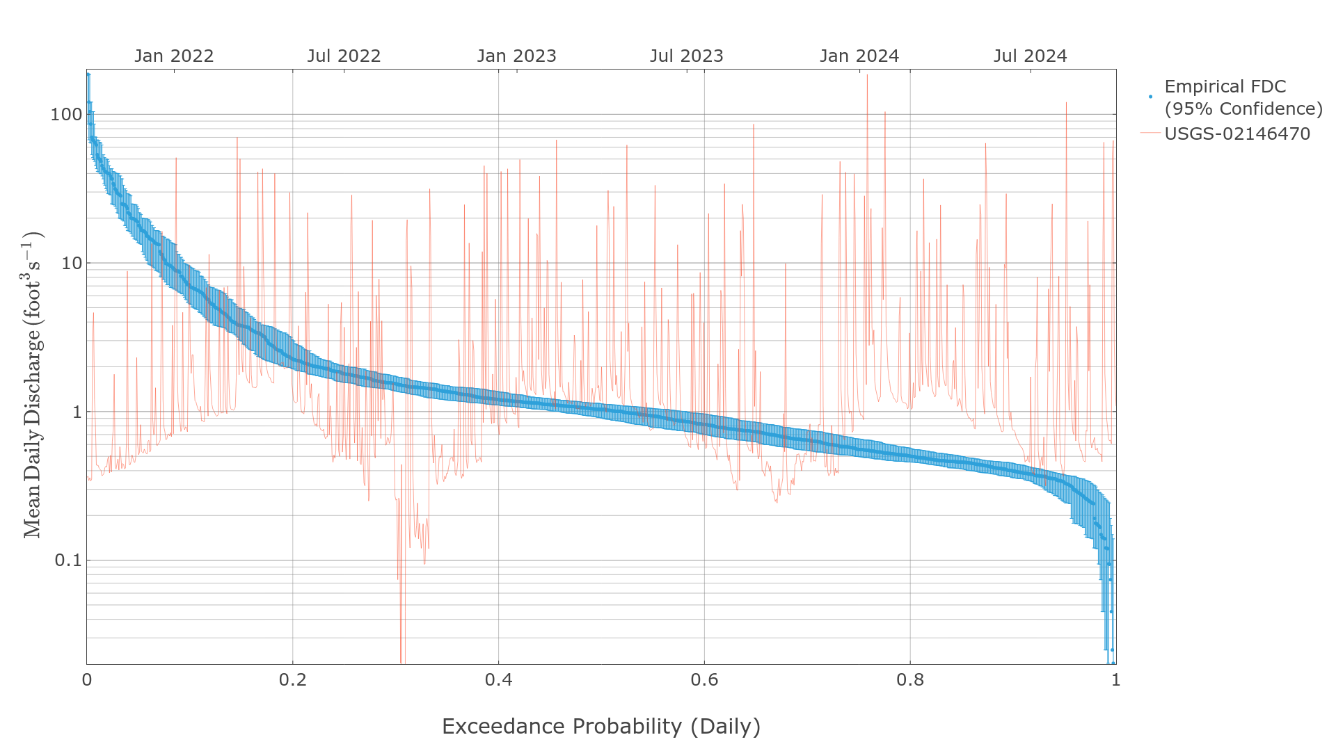
Empirical flow duration curves use simple rank ordering to generate distributions of data. The following examples require the hydrotools.nwis_client package to retrieve observed streamflow data.
# Required imports
import pandas as pd
import hydrotools.metrics.flow_duration_curve as fdc
from hydrotools.nwis_client.iv import IVDataService

# Get data and preprocess
client = IVDataService()
df = client.get(
    sites="02146470",
    startDT="2023-10-01T00:00Z",
    endDT="2024-09-30T23:59Z"
    )
df = df.drop_duplicates(["value_time"]).set_index("value_time")
df = df[["value"]].resample("1d").mean()

# Generate flow duration curve
probabilities, values = fdc.empirical_flow_duration_curve(df["value"])

# Generate 95% confidence intervals
_, boundaries = fdc.bootstrap_flow_duration_curve(
    df["value"],
    quantiles=[0.025, 0.975]
    )

# Look at the data
print(pd.DataFrame({
    "exceedance_probability": probabilities,
    "streamflow_cfs": values,
    "lower_estimate_95CI": boundaries[0],
    "upper_estimate_95CI": boundaries[1]
}).head())
Output
   exceedance_probability  streamflow_cfs  lower_estimate_95CI  upper_estimate_95CI
0                0.002717      185.652603            66.613579           185.652603
1                0.005435      120.807648            63.947605           185.652603
2                0.008152      104.227921            48.191597           185.652603
3                0.010870       66.613579            39.808090           120.807648
4                0.013587       64.890656            36.865105           120.807648
Log Pearson Type-III Flow Duration Curve
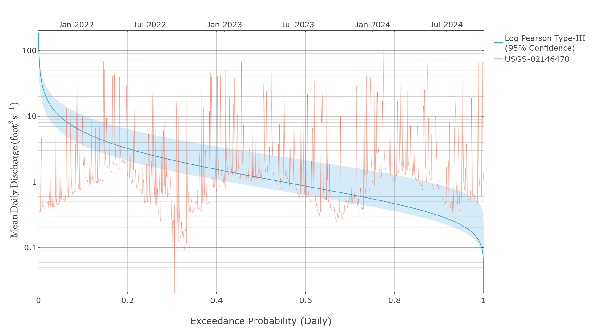
The log Pearson Type-III distribution is commonly used to model flow duration curves, especially for annual peak series. The following examples require the hydrotools.nwis_client package to retrieve observed streamflow data.
# Required imports
import pandas as pd
import hydrotools.metrics.flow_duration_curve as fdc
from hydrotools.nwis_client.iv import IVDataService

# Get data and preprocess
client = IVDataService()
df = client.get(
    sites="02146470",
    startDT="2023-10-01T00:00Z",
    endDT="2024-09-30T23:59Z"
    )
df = df.drop_duplicates(["value_time"]).set_index("value_time")
df = df[["value"]].resample("1d").mean()

# Generate flow duration curve
#  Note the log Pearson Type-III cannot handle zero values.
probabilities, values = fdc.pearson_flow_duration_curve(
    df.loc[df["value"] > 0.0, "value"])

# Generate 95% confidence intervals
_, boundaries = fdc.bootstrap_flow_duration_curve(
    df.loc[df["value"] > 0.0, "value"],
    quantiles=[0.025, 0.975],
    fdc_generator=fdc.pearson_flow_duration_curve
    )

# Look at the data
print(pd.DataFrame({
    "exceedance_probability": probabilities,
    "streamflow_cfs": values,
    "lower_estimate_95CI": boundaries[0],
    "upper_estimate_95CI": boundaries[1]
}).head())
Output
   exceedance_probability  streamflow_cfs  lower_estimate_95CI  upper_estimate_95CI
0                0.003716      185.652557            66.613571           185.652557
1                0.003787      182.314682            65.599373           182.378235
2                0.003860      179.036835            64.600616           179.161758
3                0.003934      175.817902            63.617050           176.001938
4                0.004009      172.656952            62.648510           172.897842
Flow Duration Curve Metrics
The flow_duration_curve module also includes methods to compute common flow duration curve metrics.
# Get data and preprocess
client = IVDataService()
df = client.get(
    sites="02146470",
    startDT="2023-10-01T00:00Z",
    endDT="2024-09-30T23:59Z"
    )
df = df.drop_duplicates(["value_time"]).set_index("value_time")

# Change this step to resample to relevant frequencies
#   This example uses mean daily flow. So, derived exeedances and
#   and recurrences will refer to the "Daily Exeedance Probability" and
#   "Daily Recurrence Interval".
df = df[["value"]].resample("1d").mean()

# Generate flow duration curve
probabilities, values = fdc.empirical_flow_duration_curve(df["value"])

# Generate 95% confidence intervals
_, boundaries = fdc.bootstrap_flow_duration_curve(
    df["value"],
    quantiles=[0.025, 0.975]
    )

# Interpolate values for specific exceedance probabilities
exceedance_probabilities = [0.01, 0.5, 0.67]
exceedance_values = fdc.interpolate_exceedance_values(
    points=exceedance_probabilities,
    probabilities=probabilities,
    values=values
)

# Get corresponding confidence intervals
lower_exceedance_values = fdc.interpolate_exceedance_values(
    points=exceedance_probabilities,
    probabilities=probabilities,
    values=boundaries[0]
)
upper_exceedance_values = fdc.interpolate_exceedance_values(
    points=exceedance_probabilities,
    probabilities=probabilities,
    values=boundaries[1]
)

# Interpolate values for specific recurrence intervals
recurrence_intervals = [1.5, 10.0, 100.0]
recurrence_values = fdc.interpolate_recurrence_values(
    points=recurrence_intervals,
    probabilities=probabilities,
    values=values
)

# Get corresponding confidence intervals
lower_recurrence_values = fdc.interpolate_recurrence_values(
    points=recurrence_intervals,
    probabilities=probabilities,
    values=boundaries[0]
)
upper_recurrence_values = fdc.interpolate_recurrence_values(
    points=recurrence_intervals,
    probabilities=probabilities,
    values=boundaries[1]
)

# Generate standard flow variability metrics
flow_variability = fdc.richards_flow_responsiveness(
    probabilities,
    values
)
flow_variability_low_estimate = fdc.richards_flow_responsiveness(
    probabilities,
    boundaries[0]
)
flow_variability_upper_estimate = fdc.richards_flow_responsiveness(
    probabilities,
    boundaries[1]
)

# View results
print("DAILY EXCEEDANCE PROBABILITIES")
print("==============================")
print(pd.DataFrame({
    "exceedance_probability": exceedance_probabilities,
    "exceedance_value": exceedance_values,
    "lower_estimate_95CI": lower_exceedance_values,
    "upper_estimate_95CI": upper_exceedance_values
}),"\n")
print("DAILY RECURRENCE INTERVALS")
print("==========================")
print(pd.DataFrame({
    "recurrence_interval": recurrence_intervals,
    "recurrence_value": recurrence_values,
    "lower_estimate_95CI": lower_recurrence_values,
    "upper_estimate_95CI": upper_recurrence_values
}),"\n")
print("RICHARDS FLOW VARIABILITY METRICS")
print("=================================")
print(pd.DataFrame([
    flow_variability,
    flow_variability_low_estimate,
    flow_variability_upper_estimate
    ], index=["nominal", "lower_CI95", "upper_CI95"]))
Output
DAILY EXCEEDANCE PROBABILITIES
==============================
   exceedance_probability  exceedance_value  lower_estimate_95CI  upper_estimate_95CI
0                    0.01         78.650168            42.490812           141.558033
1                    0.50          1.034132             0.861215             1.187361
2                    0.67          0.670954             0.555178             0.820956

DAILY RECURRENCE INTERVALS
==========================
   recurrence_interval  recurrence_value  lower_estimate_95CI  upper_estimate_95CI
0                  1.5          0.674086             0.556111             0.848877
1                 10.0          9.806313             6.054264            14.848021
2                100.0         78.650168            42.490812           141.558033

RICHARDS FLOW VARIABILITY METRICS
=================================
                10R90     20R80     25R75       .5S       .6S        .8S       CVLF5
nominal     24.456346  5.222382  3.274392  1.213142  2.072303   9.094914    4.403239
lower_CI95  16.956743  3.809411  3.054882  1.145003  1.491005   6.615329  144.413910
upper_CI95  32.290005  7.858763  3.805921  1.590946  3.350040  12.117785    2.474570
Release history Release notifications | RSS feed


Download files
Download the file for your platform. If you're not sure which to choose, learn more about installing packages.
Source Distribution
Built Distribution
Filter files by name, interpreter, ABI, and platform.
If you're not sure about the file name format, learn more about wheel file names.
Copy a direct link to the current filters
File details
Details for the file hydrotools_metrics-2.2.0.tar.gz.
File metadata
- Download URL: hydrotools_metrics-2.2.0.tar.gz
- Upload date:
- Size: 38.0 kB
- Tags: Source
- Uploaded using Trusted Publishing? No
- Uploaded via: twine/6.1.0 CPython/3.12.2
File hashes
| Algorithm | Hash digest | |
|---|---|---|
| SHA256 |
9c6c212f5abc38d18b2826932a1c819cf35a7d27d574693edfed2ffdf1aad16a
|
|
| MD5 |
579412bd49c5a4d6d22a01087442fe8d
|
|
| BLAKE2b-256 |
083622ebdbe4d253ef82a888b8f9cd7bf6be45ac3e53bc09d1e0d8fbf7d1f1e0
|
File details
Details for the file hydrotools_metrics-2.2.0-py3-none-any.whl.
File metadata
- Download URL: hydrotools_metrics-2.2.0-py3-none-any.whl
- Upload date:
- Size: 29.1 kB
- Tags: Python 3
- Uploaded using Trusted Publishing? No
- Uploaded via: twine/6.1.0 CPython/3.12.2
File hashes
| Algorithm | Hash digest | |
|---|---|---|
| SHA256 |
2d8cdf8a341f43ace1dd9b93d01eb10e2e9068aa8eec370782eaa757bc18741a
|
|
| MD5 |
085110fe5c0800104c968fc8eff0d52b
|
|
| BLAKE2b-256 |
aa10de3b34aaa67edc860496bb74df59152471bf67e97805a7ed9b225b19e765
|


