
Classical and Quantum Ideal Gases



Ideal-gases is a collection of numerical solvers for:
- classical and quantum Euler inviscid gases,
- classical and quantum 1-D Navier–Stokes–Fourier (NSF) viscous gases,
- classical and quantum 1-D BGK, Shakhov, and ES-BGK solvers for rarefied gases,
- C++ kernels for the polylogarithm and fugacity inversion used to resolve the quantum equation of state.
This repository ports the MATLAB implementation found in this NTU thesis to Python 3.11. The polylog function has been ported from the MATLAB implementation to C++, fugacity inversion is a C++ kernel alongside it. For Euler equations, the Toro exact Riemann solver has been extended to support Fermi–Dirac (FD), Bose–Einstein (BE), and Maxwell–Boltzmann (MB) statistics following the example found in the anexes of this NTU thesis.
Requirements
Building from source additionally requires a C++17 compiler. See DEVELOPER_GUIDE.md.
Installation
pip install ideal-gases
For plotting (euler plot, interactive explorers):
pip install ideal-gases[plot]
For QBE-matched Shakhov (matched_qbe):
pip install ideal-gases[tables]
For progress bars (--progress on the numerical CLIs, and the solver progress= flag):
pip install ideal-gases[progress]
After install, the euler, nsf, bgk, shakhov, and es command-line tools are available.
Interactive mode
Launch matplotlib widget explorers to build custom Riemann problems with sliders, statistic toggles (quantum), and Save/Reset controls. Y-axis limits autoscale automatically on each update.
euler interactive classical
euler interactive quantum
Seed the initial state from CLI flags or a JSON config (same fields as euler solve):
euler interactive classical --gamma 1.4 --t-end 0.5 --nx 101
euler interactive quantum --rho-l 2 --t-l 1.5 --n 3 --h 0.5
euler interactive classical --config case.json
Optional domain flags (--x-min, --x-max, --x0, --nx) default to an interactive Sod-tube layout (x in [-10, 10], discontinuity at x0=0, nx=1024). Use -f path.png to set the Save button target; nothing is written until you click Save.
Example usage
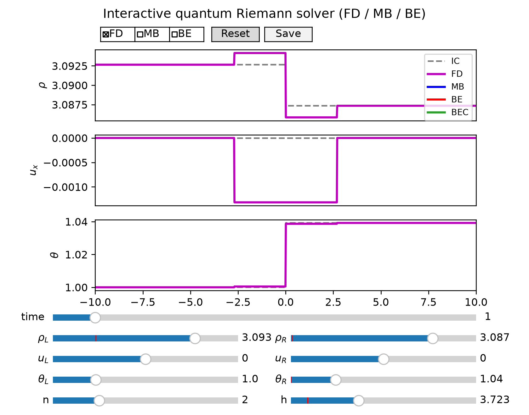
euler interactive quantum
Outputs a Sod shock tube problem resolved with a quantum Euler solver for all statistics. We deactivate the solutions of MB and BE to focus on the FD solution. Using the slider, we can vary the left and right states and the thermal scale parameter h and the number of degrees of freedom n of the gas.
In Fig. 5 of Hu and Jing (2010), a fictitious 2-d fermi gas degenerate regime is used to prove the accuracy of Kinetic Flux Vector Splitting schemes for quantum Euler equations. Using the interactive mode, we set n : 2 and set the left and right states ($\rho,u,\theta$). Using the h slider, we found that the degenerate gas is resolved approximately for h $\approx$ 3.71.
As show in the following figure:
Command-line mode
Compute exact solution profiles, save plots to PNG, and write CSV/JSON files with the solution fields.
Classical Sod shock tube
euler solve classical \
  --rho-l 1 --u-l 0 --p-l 1 \
  --rho-r 0.125 --u-r 0 --p-r 0.1 \
  --t-end 0.25 --gamma 1.4 \
  --nx 101 -o sod.csv
Quantum Euler
euler solve quantum \
  --rho-l 1 --u-l 0 --t-l 1 \
  --rho-r 0.125 --u-r 0 --t-r 0.25 \
  --t-end 0.20 --n 2 --h 0.1 --statistic FD \
  -o euler_fd.csv
Write separate files for FD, MB, and BE with --all-statistics (e.g. euler_case7_FD.csv, euler_case7_MB.csv, euler_case7_BE.csv):
euler solve quantum ... --all-statistics -o euler_case7
Equilibrium inversions
Compute the fugacity from density and temperature:
euler fugacity --rho 1.0 --theta 1.0 --n 3 --h 1.0 --statistic FD
Recover fugacity, temperature and pressure from density and internal energy:
euler moments --rho 1.0 --e 1.5 --n 3 --h 1.0 --statistic FD
Use -o result.json to write JSON output instead of printing to stdout.
Built-in benchmarks
euler toro 1 -o toro_test1.csv
euler list --toro

euler quantum-example 7 --all-statistics -o euler_eg7
euler list --quantum
JSON config files
Define a problem in JSON and run it with euler run or pass --config to euler solve:
euler run --config case.json
euler solve classical --config case.json -o override.csv
Example case.json:
{
  "mode": "quantum",
  "left": {"rho": 1.0, "u": 0.0, "theta": 1.0},
  "right": {"rho": 0.125, "u": 0.0, "theta": 0.25},
  "t_end": 0.20,
  "n": 2.0,
  "h": 0.1,
  "statistic": "FD",
  "all_statistics": true,
  "format": "json",
  "output": "euler_case7",
  "domain": {"x_min": 0.0, "x_max": 1.0, "x0": 0.5, "nx": 101}
}
Use --format json (or a .json output path) for JSON instead of CSV. CLI flags override values from the config file.
Visualization
Save a classical Sod shock tube figure:
euler plot classical \
  --rho-l 1 --u-l 0 --p-l 1 \
  --rho-r 0.125 --u-r 0 --p-r 0.1 \
  --t-end 0.2 --gamma 1.4 --nx 101 \
  -f sod.png
Plot a single quantum statistic or compare FD/MB/BE:
euler plot quantum \
  --rho-l 1 --u-l 0 --t-l 1 \
  --rho-r 0.125 --u-r 0 --t-r 0.25 \
  --t-end 0.20 --n 2 --h 0.1 --statistic FD \
  -f qfd.png

euler plot quantum-example 7 --all-statistics -f eg7
With --all-statistics, -f eg7 writes eg7_panels.png (3×6 grid) and eg7_comparison.png (overlay). Use --layout panels|comparison|both to select one or both (default: both). Add --show for an interactive window, or -o to export CSV/JSON in the same run.
Example usage
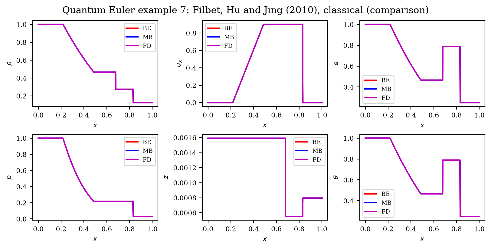
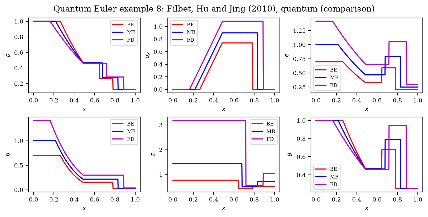
In Filbet, Hu and Jing (2010), the authors use a Sod shock tube initial condition with a fictitious 2-d fermi and bose gas to prove the accuracy of their numerical scheme in classical and quantum hydronamic regimes. These are examples 7 and 8, respectively, in the CLI plot tool.
euler plot quantum-example 7 --all-statistics -f sod_2d_gas_classical --layout comparison --show
yields the following plot:
euler plot quantum-example 8 --all-statistics -f sod_2d_gas_quantum --layout comparison --show
yields the following plot:
NSF, BGK, Shakhov, and ES CLIs
The nsf, bgk, shakhov, and es commands mirror euler’s run / solve / plot verbs (no interactive mode, Toro presets, or --all-statistics). They write cell-centered profiles. solve and run require -o. plot requires -f or --show.
nsf solve classical --kn 1e-3 --t-end 0.1 --dim 3 -o nsf.csv
nsf solve quantum --kn 1e-3 --h 1 --statistic FD -o qnsf.csv
nsf solve quantum --matched-qbe --kn 1 --statistic FD -o qnsf-matched.csv
nsf run --config case.json
nsf plot classical --kn 1e-3 --t-end 0.1 -f nsf.png
nsf plot --input nsf.csv -f nsf.png

bgk solve classical --kn 1e-3 --nv 64 -o bgk.csv
shakhov solve quantum --matched-qbe --kn 1 --statistic FD -o matched.csv

es solve classical --kn 1e-3 --t-end 0.1 --b -0.5 -o es.csv
es solve quantum --kn 1e-3 --h 1 --statistic FD -o qes.csv
es solve quantum --matched-qbe --kn 1 --statistic FD -o es-matched.csv
Classical Sod defaults are (ρ,u,p) = (1,0,1) / (0.125,0,0.1). Quantum defaults use temperatures (1, 0.8) (the same p/ρ with R = 1). The spatial grid is cell-centered (nx=200 by default). Kinetic solvers (bgk, shakhov, es) default to nv=128 velocity nodes; pass --nv to override (the examples above that pass --nv 64 do so on purpose). CSV files start with # key=value metadata, then a header x,rho,u,T,p,q (quantum adds z).
es fixes dim=3. Classical Holway b defaults to -0.5 and is ignored on es solve quantum when --matched-qbe is set. QBE-matched NSF and Shakhov (--matched-qbe) freeze dim=3, idof=0 and require FD or BE. NSF calls nsf_matched_qbe; Shakhov calls shakhov_matched_qbe. Matched ES-BGK is Fermi only (FD) and calls es_matched_qbe. BGK has no matching flag.
Example numerical JSON (kn is required; nsf run will not invent it from an Euler-only file):
{
  "mode": "classical",
  "kn": 0.001,
  "dim": 3,
  "idof": 0,
  "left": {"rho": 1.0, "u": 0.0, "p": 1.0},
  "right": {"rho": 0.125, "u": 0.0, "p": 0.1},
  "t_end": 0.1,
  "domain": {"x_min": 0.0, "x_max": 1.0, "x0": 0.5, "nx": 200},
  "output": "nsf.csv"
}
Python module
Import ideal_gases to compute classical and quantum Euler, NSF, and ES-BGK solutions in your own scripts.
Classical Euler
import numpy as np
from ideal_gases import classical_euler

x = np.linspace(0.0, 1.0, 101)
result = classical_euler(
    rho_l=1.0,
    u_l=0.0,
    p_l=1.0,
    rho_r=0.125,
    u_r=0.0,
    p_r=0.1,
    t_end=0.2,
    gamma=1.4,
    x=x,
    x0=0.5,
)
Quantum Euler (FD / BE / MB)
Left and right states are given in terms of density rho, velocity u, and temperature theta (written t in the API). The solver converts these to effective pressures via the quantum EOS, then applies the Toro exact Riemann solver.
import numpy as np
from ideal_gases import quantum_euler

x = np.linspace(0.0, 1.0, 101)
result = quantum_euler(
    rho_l=1.0,
    u_l=0.0,
    t_l=1.0,
    rho_r=0.125,
    u_r=0.0,
    t_r=0.25,
    t_end=0.20,
    n=2.0,          # degrees of freedom; gamma = (n+2)/n
    h=0.1,          # thermal scale parameter
    statistic="FD", # "FD", "BE", or "MB"
    x=x,
    x0=0.5,
)
This returns a RiemannResult object that contains the solution fields: x, rho, ux, p, e, z (fugacity), t (temperature), mach, entropy.
In the classical limit, MB statistics with h → 0 recover the ideal-gas behaviour (pressures p = rho * theta).
Classical NSF
1-D Navier–Stokes–Fourier for a polytropic ideal gas. Same Sod left/right states as the classical Euler example; dim in {1, 2, 3} is the translational dimension and idof (default 0, monatomic) is the internal DoF, so γ = (n+2)/n with n = dim + idof. For air-like γ = 1.4 use dim=3, idof=2. Classical Euler remains a γ-law Riemann solver (gamma=). kn is the Knudsen number used by the Chapman–Enskog closure μ = kn ρ T. Default Prandtl number is Eucken 4γ / (9γ - 5) (2/3 when n = 3); pass pr= to override.
import numpy as np
from ideal_gases import classical_nsf

x = np.linspace(0.0, 1.0, 101)
result = classical_nsf(
    rho_l=1.0,
    u_l=0.0,
    p_l=1.0,
    rho_r=0.125,
    u_r=0.0,
    p_r=0.1,
    t_end=0.2,
    dim=3,
    kn=0.01,
    idof=2.0,  # γ = 1.4; omit or 0 for monatomic γ = 5/3
    x=x,
    x0=0.5,
)
This returns a ClassicalNSFResult object that contains the cell-centered fields: rho, u, t (temperature), p, q (heat flux).
Classical Shakhov
Reduced (g, h) asymptotic-preserving DVM for 1-D flow of a 2-D or 3-D polytropic gas. Time is first-order IMEX. Default closures match classical NSF (τ = kn, Eucken Pr = 4γ / (9γ - 5)). Optional idof (default 0) sets γ = (n+2)/n with n = dim + idof; h holds perpendicular translational energy plus internal energy. Optional viscosity and prandtl hooks replace those closures (for example Boltzmann CE μ ∝ T^ω); there is no conductivity hook.
import numpy as np
from ideal_gases import classical_shakhov

x = np.linspace(0.0, 1.0, 101)
result = classical_shakhov(
    rho_l=1.0,
    u_l=0.0,
    p_l=1.0,
    rho_r=0.125,
    u_r=0.0,
    p_r=0.1,
    t_end=0.2,
    dim=3,
    kn=0.01,
    idof=2.0,  # γ = 1.4; omit or 0 for monatomic γ = 5/3
    x=x,
    x0=0.5,
    nv=64,
    xi_max=8.0,
)
This returns the same ClassicalNSFResult fields as classical_nsf.
Classical BGK
Reduced (g, h) asymptotic-preserving DVM that relaxes to the Maxwellian (Pr = 1). Time is first-order IMEX. Default viscosity is μ = kn ρ T (τ = kn). Optional idof (default 0) is the same polytropic parameter as Shakhov/NSF. Optional viscosity replaces that closure; there is no Prandtl hook, because BGK cannot independently match Boltzmann heat conductivity.
import numpy as np
from ideal_gases import classical_bgk

x = np.linspace(0.0, 1.0, 101)
result = classical_bgk(
    rho_l=1.0,
    u_l=0.0,
    p_l=1.0,
    rho_r=0.125,
    u_r=0.0,
    p_r=0.1,
    t_end=0.2,
    dim=3,
    kn=0.01,
    idof=2.0,  # γ = 1.4; omit or 0 for monatomic γ = 5/3
    x=x,
    x0=0.5,
    nv=64,
    xi_max=8.0,
)
This returns the same ClassicalNSFResult fields as classical_nsf.
Classical ES-BGK
1-D Holway ES-BGK on a full 3-D velocity lattice (dim=3 only). Default monatomic tuning is b = -1/2, μ = kn ρ T, and τ = (1-b) μ / p (Eucken Pr = 2/3).
import numpy as np
from ideal_gases import classical_es_bgk

x = np.linspace(0.0, 1.0, 101)
result = classical_es_bgk(
    rho_l=1.0,
    u_l=0.0,
    p_l=1.0,
    rho_r=0.125,
    u_r=0.0,
    p_r=0.1,
    t_end=0.2,
    kn=0.01,
    dim=3,
    b=-0.5,
    x=x,
    x0=0.5,
    nv=64,
    xi_max=8.0,
)
This returns a ClassicalESResult (rho, u, t, p, q).
Quantum NSF (FD / BE / MB)
1-D Navier–Stokes–Fourier with the quantum EOS. Same left/right states as the quantum Euler example; dim is the translational dimension (Euler's n in the monatomic case), and idof (default 0) sets γ = (n+2)/n with n = dim + idof. kn sets the Chapman–Enskog viscosity μ = kn p(z). Default conductivity uses Pr_z = Pr_Eucken R(z) with the same Eucken factor as classical NSF. Quantum Euler uses a single n (set n = dim + idof for a polytropic comparison).
import numpy as np
from ideal_gases import quantum_nsf

x = np.linspace(0.0, 1.0, 101)
result = quantum_nsf(
    rho_l=1.0,
    u_l=0.0,
    t_l=1.0,
    rho_r=0.125,
    u_r=0.0,
    t_r=0.25,
    t_end=0.20,
    dim=3,
    h=0.1,
    kn=0.01,
    idof=2.0,  # γ = 1.4; omit or 0 for monatomic
    statistic="FD", # "FD", "BE", or "MB"
    x=x,
    x0=0.5,
)
This returns a QuantumNSFResult object (NSFResult is an alias) that contains: rho, u, t, p, z (fugacity), q (heat flux).
Quantum Shakhov (FD / BE / MB)
Reduced (g, h_r) asymptotic-preserving DVM for 1-D flow of a 2-D or 3-D polytropic gas. Time is first-order IMEX. Default closures are quantum CE (τ = kn, Pr_z = Pr_Eucken R(z); 2/3 R(z) when n = 3). Optional idof (default 0) sets γ = (n+2)/n with n = dim + idof; h_r holds perpendicular translational energy plus internal energy (Diaz extra momenta). Optional viscosity and prandtl hooks replace those closures (for example QBE tables); there is no conductivity hook.
import numpy as np
from ideal_gases import quantum_shakhov

x = np.linspace(0.0, 1.0, 101)
result = quantum_shakhov(
    rho_l=1.0,
    u_l=0.0,
    t_l=1.0,
    rho_r=0.125,
    u_r=0.0,
    t_r=0.25,
    t_end=0.20,
    dim=3,
    h=0.1,
    kn=0.01,
    idof=2.0,  # γ = 1.4; omit or 0 for monatomic
    statistic="FD",  # "FD", "BE", or "MB"
    x=x,
    x0=0.5,
    nv=64,
    xi_max=8.0,
)
This returns the same QuantumNSFResult fields as quantum_nsf.
Quantum QBE-matched NSF, Shakhov, and ES-BGK
1-D flow of a 3-D monatomic Fermi or Bose gas with Wu CE transport tables Φ_μ(z, θ), Φ_κ(z, θ). nsf_matched_qbe is quantum_nsf and shakhov_matched_qbe is quantum_shakhov, each with dim=3, idof=0, and closures
μ = Kn √T Φ_μ(z, θ), κ = Kn (15/4) √T Φ_κ(z, θ), Pr_z = Pr_Q / R(z)
es_matched_qbe is the same 3-D monatomic setup for Fermi gases only. Holway b(z) = 1 - R(z)/Pr_Q(z) and τ = (1-b) μ_Q / p follow Wu Section 4. Bose gases stay on shakhov_matched_qbe.
θ = T/T_a is a collision-kernel parameter (default 0 is the s-wave limit), not the hydrodynamic temperature in √T. Requires pip install ideal-gases[tables]. Maxwell–Boltzmann is not tabulated.
import numpy as np
from ideal_gases.matched_qbe import es_matched_qbe, nsf_matched_qbe, shakhov_matched_qbe

x = np.linspace(0.0, 1.0, 101)
kin = shakhov_matched_qbe(
    rho_l=1.0,
    u_l=0.0,
    t_l=1.0,
    rho_r=0.4,
    u_r=0.0,
    t_r=0.6,
    t_end=0.10,
    h=3.0,
    kn=0.01,
    statistic="BE",  # "FD" or "BE"
    theta=0.0,       # T/T_a
    x=x,
    x0=0.5,
    nv=64,
    xi_max=8.0,
)
nsf = nsf_matched_qbe(
    rho_l=1.0,
    u_l=0.0,
    t_l=1.0,
    rho_r=0.4,
    u_r=0.0,
    t_r=0.6,
    t_end=0.10,
    h=3.0,
    kn=0.01,
    statistic="BE",
    theta=0.0,
    x=x,
    x0=0.5,
)
es = es_matched_qbe(
    rho_l=1.0,
    u_l=0.0,
    t_l=1.0,
    rho_r=0.4,
    u_r=0.0,
    t_r=0.6,
    t_end=0.10,
    h=3.0,
    kn=0.01,
    statistic="FD",  # Fermi only
    theta=0.0,
    x=x,
    x0=0.5,
    nv=64,
    xi_max=8.0,
)
This returns the same QuantumNSFResult fields as quantum_nsf.
Quantum ES-BGK (FD / BE / MB)
1-D quantum ES-BGK on a full 3-D velocity lattice (dim=3 only). Default transport is Chapman–Enskog μ = kn p(z) with Holway b = -1/2. Pass viscosity for a custom closure; QBE-matched tables use es_matched_qbe above.
import numpy as np
from ideal_gases import quantum_es_bgk

x = np.linspace(0.0, 1.0, 101)
result = quantum_es_bgk(
    rho_l=1.0,
    u_l=0.0,
    t_l=1.0,
    rho_r=0.125,
    u_r=0.0,
    t_r=0.25,
    t_end=0.20,
    dim=3,
    h=0.1,
    kn=0.01,
    statistic="FD",  # "FD", "BE", or "MB"
    x=x,
    x0=0.5,
    nv=64,
    xi_max=8.0,
)
This returns the same QuantumNSFResult fields as quantum_nsf.
Quantum BGK (FD / BE / MB)
Reduced (g, h_r) asymptotic-preserving DVM that relaxes to the FD/BE/MB equilibrium (Pr_z = 1). Time is first-order IMEX. Default viscosity is μ = kn p(z) (τ = kn). Optional idof (default 0) is the same polytropic parameter as Shakhov/NSF. Optional viscosity replaces that closure ((rho, temp, z) → μ); there is no Prandtl hook, because BGK cannot independently match heat conductivity.
import numpy as np
from ideal_gases import quantum_bgk

x = np.linspace(0.0, 1.0, 101)
result = quantum_bgk(
    rho_l=1.0,
    u_l=0.0,
    t_l=1.0,
    rho_r=0.125,
    u_r=0.0,
    t_r=0.25,
    t_end=0.20,
    dim=3,
    h=0.1,
    kn=0.01,
    idof=2.0,  # γ = 1.4; omit or 0 for monatomic
    statistic="FD",  # "FD", "BE", or "MB"
    x=x,
    x0=0.5,
    nv=64,
    xi_max=8.0,
)
This returns the same QuantumNSFResult fields as quantum_nsf.
Equilibrium inversions
Given density and temperature, recover the fugacity:
from ideal_gases import find_fugacity

z = find_fugacity(rho=1.0, T=1.0, dim=3, h=1.0, eta=-1)
Given density and internal energy, recover fugacity, temperature and pressure:
from ideal_gases import find_moments

z, T, p = find_moments(rho=1.0, e=2.5, dim=3, h=1.0, eta=-1, idof=2.0)
The eta parameter selects the statistic: -1 Fermi, 0 classical (Maxwell-Boltzmann), +1 Bose. Optional idof (default 0) is the internal DoF; thermodynamic closures use n = dim + idof.
Given density and the mass-weighted second-moment tensor W, recover the ES fugacity and the tensor λ. dim is the velocity-space dimension (2 or 3). This path uses the C++ find_fugacity_es kernel and does not take idof.
import numpy as np
from ideal_gases import find_fugacity_anisotropic

w = np.eye(3)
z, lam = find_fugacity_anisotropic(rho=1.0, w=w, dim=3, h=1.0, eta=-1)
Polylogarithm module
Building from source compiles three C++ extensions: _polylog, _find_fugacity, and _find_fugacity_es. polylog(n, z) uses the Fukushima minimax Fermi–Dirac / Bose–Einstein integrals for supported half-integer orders on z < 0 and 0 < z < 1, with Bhagat / integer analytic branches as fallback. find_fugacity and find_fugacity_anisotropic call the fugacity kernels.
We can use the polylogarithm module on our scripts as follows:
import numpy as np
from ideal_gases import polylog

polylog(2, 0.5)                         # scalar
polylog(1.5, np.linspace(0.2, 0.9, 50)) # array
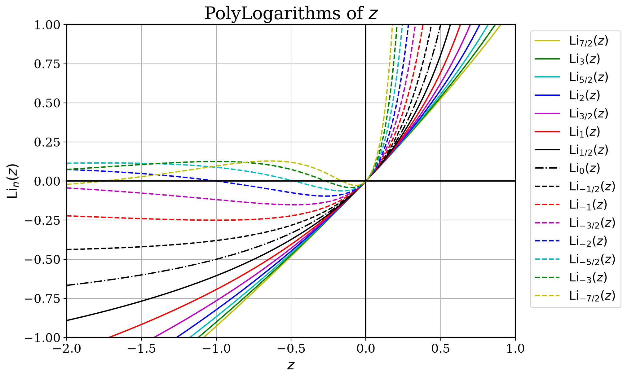
We can plot the polylogarithm function to verify the accuracy of the implementation for integer and half-integer orders as follows:
uv run python scripts/plot_polylogarithms.py --output figures/polylogarithms.png
Omitting --output writes PolyLogPlot.png in the repo root. The command above yields the following plot:
Public API
from ideal_gases import (
    G,
    ClassicalESResult,
    ClassicalNSFResult,
    QuantumNSFResult,
    RiemannResult,
    DEFAULT_HOLWAY_B_3D,
    adiabatic_index,
    classical_euler,
    classical_es_bgk,
    classical_nsf,
    classical_bgk,
    classical_shakhov,
    equilibrium_moments,
    eucken_prandtl,
    find_fugacity,
    find_fugacity_anisotropic,
    find_moments,
    polylog,
    quantum_euler,
    quantum_es_bgk,
    quantum_nsf,
    quantum_bgk,
    es_matched_qbe,
    matched_qbe,
    quantum_shakhov,
    w_from_pressure,
)
| Symbol | Role |
|---|---|
polylog(n, z) |
Fast C++ polylogarithm (Fukushima + Bhagat/integer fallback) |
adiabatic_index(n) |
Returns γ = (n + 2) / n |
eucken_prandtl(n) |
Eucken Pr = 4γ / (9γ - 5); 2/3 at n = 3 |
classical_euler(...) |
Classical ideal-gas exact Euler Riemann solver |
quantum_euler(...) |
Quantum EOS + Toro exact Euler Riemann solver |
classical_nsf(...) |
1-D classical Navier–Stokes–Fourier solver (idof for polytropic γ) |
classical_bgk(...) |
1-D classical BGK AP DVM (dim in {2, 3}, idof for polytropic γ) |
classical_shakhov(...) |
1-D classical Shakhov AP DVM (dim in {2, 3}, idof for polytropic γ) |
classical_es_bgk(...) |
1-D classical Holway ES-BGK (dim=3, full 3-D velocity lattice) |
quantum_nsf(...) |
1-D quantum Navier–Stokes–Fourier solver (idof for polytropic γ) |
quantum_bgk(...) |
1-D quantum BGK AP DVM (dim in {2, 3}, idof for polytropic γ) |
quantum_shakhov(...) |
1-D quantum Shakhov AP DVM (dim in {2, 3}, idof for polytropic γ) |
quantum_es_bgk(...) |
1-D quantum ES-BGK (dim=3, full 3-D velocity lattice) |
matched_qbe |
QBE-matched module (from ideal_gases import matched_qbe) |
nsf_matched_qbe(...) |
QBE-matched 3-D monatomic NSF (FD/BE, Wu Φ_μ, Φ_κ tables); import from ideal_gases.matched_qbe |
shakhov_matched_qbe(...) |
QBE-matched 3-D monatomic Shakhov (FD/BE, Wu Φ_μ, Φ_κ tables); import from ideal_gases.matched_qbe |
es_matched_qbe(...) |
QBE-matched 3-D monatomic ES-BGK (FD only, Wu §4 b(z)); also from ideal_gases import es_matched_qbe or ideal_gases.matched_qbe |
RiemannResult |
Euler solution profiles on the spatial grid |
ClassicalNSFResult |
Classical NSF fields (rho, u, t, p, q) |
ClassicalESResult |
Classical ES-BGK fields (rho, u, t, p, q) |
QuantumNSFResult |
Quantum NSF fields (rho, u, t, p, z, q) |
G(n, z, eta) |
Bose / Fermi / classical partition function |
equilibrium_moments(z, T, ...) |
Forward map (z, T) → (ρ, e) |
find_fugacity(rho, T, ...) |
Invert (ρ, T) → z (C++ _find_fugacity) |
find_fugacity_anisotropic(rho, w, ...) |
Invert (ρ, W) → (z, λ) for the ES reference state (dim in {2, 3}, C++ _find_fugacity_es) |
find_moments(rho, e, ...) |
Invert (ρ, e) → (z, T, p) |
w_from_pressure(P, b, dim) |
Holway map W = (1-b) p I + b P with p = tr(P)/D |
DEFAULT_HOLWAY_B_3D |
Default Holway parameter b = -1/2 for 3-D monatomic ES-BGK |
License
MIT License. See LICENSE for the full text.
Copyright (c) 2026 Manuel A. Diaz
For building from source, tests, linting, CI, and releases, see DEVELOPER_GUIDE.md.
1 maintainer

Release files for ideal-gases 0.1.5
For a detailed explanation of source distributions (sdists) and built distributions (wheels), please see the package formats documentation.
Source distribution (sdist)
| File | Size | Uploaded | |
|---|---|---|---|
| ideal_gases-0.1.5.tar.gz | 1.0 MB | Details |
Built distributions (wheels)
| File | Reset | |||
|---|---|---|---|---|
| ideal_gases-0.1.5-cp313-cp313-manylinux_2_24_x86_64.manylinux_2_28_x86_64.whl | CPython 3.13 | CPython 3.13 | Linux glibc 2.28+ x86-64, Linux glibc 2.24+ x86-64 | Details |
| ideal_gases-0.1.5-cp313-cp313-macosx_11_0_arm64.whl | CPython 3.13 | CPython 3.13 | macOS 11.0+ ARM64 | Details |
| ideal_gases-0.1.5-cp312-cp312-manylinux_2_24_x86_64.manylinux_2_28_x86_64.whl | CPython 3.12 | CPython 3.12 | Linux glibc 2.28+ x86-64, Linux glibc 2.24+ x86-64 | Details |
| ideal_gases-0.1.5-cp312-cp312-macosx_11_0_arm64.whl | CPython 3.12 | CPython 3.12 | macOS 11.0+ ARM64 | Details |
| ideal_gases-0.1.5-cp311-cp311-manylinux_2_24_x86_64.manylinux_2_28_x86_64.whl | CPython 3.11 | CPython 3.11 | Linux glibc 2.24+ x86-64, Linux glibc 2.28+ x86-64 | Details |
| ideal_gases-0.1.5-cp311-cp311-macosx_11_0_arm64.whl | CPython 3.11 | CPython 3.11 | macOS 11.0+ ARM64 | Details |
Total release size: 4.1 MB
Release files / ideal_gases-0.1.5.tar.gz
| Download URL | ideal_gases-0.1.5.tar.gz |
|---|---|
| Size | 1.0 MB |
| Tags | Source |
|
SHA-256 checksum How to use checksums |
933c90c52ca89507b0f2ac2fa4fb9bafde271657e0bc9a9d0c0677e45f4a247e
|
|
BLAKE2b-256 checksum How to use checksums |
db385107495537cd65e60120707baf6b50db42af04c9537ce4e48ba7b5459404
|
| Upload date | |
|
Uploaded using Trusted Publishing? What is trusted publishing? |
Yes |
| Uploaded via |
twine/7.0.0 CPython/3.13.14
|
Provenance
Provenance describes where a file came from. On PyPI, provenance is shared via attestations, which provide a verifiable record of the build or publishing details. View details, limitations and caveats.


PyPI Publish Attestation
PyPI verified that this artifact, at this checksum, originated from the publisher listed below.
Signed by GitHub Actions, verified by PyPI on Sep 24, 2026.
Transparency logRelease files / ideal_gases-0.1.5-cp313-cp313-manylinux_2_24_x86_64.manylinux_2_28_x86_64.whl
| Download URL | ideal_gases-0.1.5-cp313-cp313-manylinux_2_24_x86_64.manylinux_2_28_x86_64.whl |
|---|---|
| Size | 542.6 kB |
| Tags | CPython 3.13 Linux glibc 2.24+ x86-64 Linux glibc 2.28+ x86-64 |
|
SHA-256 checksum How to use checksums |
3abd62b42029ed2947cf2af85b3d775203c2c5608df694d709a281329949d473
|
|
BLAKE2b-256 checksum How to use checksums |
7bac9ac93bffbf5eadfef32935331daf23f79a4b5a3cc597810dacf6cc82fb55
|
| Upload date | |
|
Uploaded using Trusted Publishing? What is trusted publishing? |
Yes |
| Uploaded via |
twine/7.0.0 CPython/3.13.14
|
Provenance
Provenance describes where a file came from. On PyPI, provenance is shared via attestations, which provide a verifiable record of the build or publishing details. View details, limitations and caveats.
PyPI Publish Attestation
PyPI verified that this artifact, at this checksum, originated from the publisher listed below.
Signed by GitHub Actions, verified by PyPI on Sep 24, 2026.
Transparency logRelease files / ideal_gases-0.1.5-cp313-cp313-macosx_11_0_arm64.whl
| Download URL | ideal_gases-0.1.5-cp313-cp313-macosx_11_0_arm64.whl |
|---|---|
| Size | 485.8 kB |
| Tags | CPython 3.13 macOS 11.0+ ARM64 |
|
SHA-256 checksum How to use checksums |
d34c031386e62482cd31f5294d0d537727047c32b523811662cb214014a3ca36
|
|
BLAKE2b-256 checksum How to use checksums |
0f58ca2156bf94173c262e0897a5bdca8829a44278b4a16f16d8defef41e9982
|
| Upload date | |
|
Uploaded using Trusted Publishing? What is trusted publishing? |
Yes |
| Uploaded via |
twine/7.0.0 CPython/3.13.14
|
Provenance
Provenance describes where a file came from. On PyPI, provenance is shared via attestations, which provide a verifiable record of the build or publishing details. View details, limitations and caveats.
PyPI Publish Attestation
PyPI verified that this artifact, at this checksum, originated from the publisher listed below.
Signed by GitHub Actions, verified by PyPI on Sep 24, 2026.
Transparency logRelease files / ideal_gases-0.1.5-cp312-cp312-manylinux_2_24_x86_64.manylinux_2_28_x86_64.whl
| Download URL | ideal_gases-0.1.5-cp312-cp312-manylinux_2_24_x86_64.manylinux_2_28_x86_64.whl |
|---|---|
| Size | 542.8 kB |
| Tags | CPython 3.12 Linux glibc 2.24+ x86-64 Linux glibc 2.28+ x86-64 |
|
SHA-256 checksum How to use checksums |
824163f8b73596e391588ba5469508081f73a0cac47dd3bc215477cbf9ce1a26
|
|
BLAKE2b-256 checksum How to use checksums |
b7a62844d58d15b211bca9989d79d3b143968e6467d5a1d35aa6d4f7929a0164
|
| Upload date | |
|
Uploaded using Trusted Publishing? What is trusted publishing? |
Yes |
| Uploaded via |
twine/7.0.0 CPython/3.13.14
|
Provenance
Provenance describes where a file came from. On PyPI, provenance is shared via attestations, which provide a verifiable record of the build or publishing details. View details, limitations and caveats.
PyPI Publish Attestation
PyPI verified that this artifact, at this checksum, originated from the publisher listed below.
Signed by GitHub Actions, verified by PyPI on Sep 24, 2026.
Transparency logRelease files / ideal_gases-0.1.5-cp312-cp312-macosx_11_0_arm64.whl
| Download URL | ideal_gases-0.1.5-cp312-cp312-macosx_11_0_arm64.whl |
|---|---|
| Size | 485.7 kB |
| Tags | CPython 3.12 macOS 11.0+ ARM64 |
|
SHA-256 checksum How to use checksums |
76720e96ab2df9358f11152d3fb630b6a4ff7d14cfd3dd879df5aeda44f2169b
|
|
BLAKE2b-256 checksum How to use checksums |
dc408c0596e0da42c7c70fa9c0c5ba9d23d5a16b7f56c4d31dde9eae967845a8
|
| Upload date | |
|
Uploaded using Trusted Publishing? What is trusted publishing? |
Yes |
| Uploaded via |
twine/7.0.0 CPython/3.13.14
|
Provenance
Provenance describes where a file came from. On PyPI, provenance is shared via attestations, which provide a verifiable record of the build or publishing details. View details, limitations and caveats.
PyPI Publish Attestation
PyPI verified that this artifact, at this checksum, originated from the publisher listed below.
Signed by GitHub Actions, verified by PyPI on Sep 24, 2026.
Transparency logRelease files / ideal_gases-0.1.5-cp311-cp311-manylinux_2_24_x86_64.manylinux_2_28_x86_64.whl
| Download URL | ideal_gases-0.1.5-cp311-cp311-manylinux_2_24_x86_64.manylinux_2_28_x86_64.whl |
|---|---|
| Size | 542.3 kB |
| Tags | CPython 3.11 Linux glibc 2.24+ x86-64 Linux glibc 2.28+ x86-64 |
|
SHA-256 checksum How to use checksums |
c39e47a22ae6853b185eafd95f2efa33bf1152dbee852ba73ef2ee2e33957dda
|
|
BLAKE2b-256 checksum How to use checksums |
457c7f28dfe1ed73206190e85ed4587eb73d99929492bf5cb619788bfe6bbdfd
|
| Upload date | |
|
Uploaded using Trusted Publishing? What is trusted publishing? |
Yes |
| Uploaded via |
twine/7.0.0 CPython/3.13.14
|
Provenance
Provenance describes where a file came from. On PyPI, provenance is shared via attestations, which provide a verifiable record of the build or publishing details. View details, limitations and caveats.
PyPI Publish Attestation
PyPI verified that this artifact, at this checksum, originated from the publisher listed below.
Signed by GitHub Actions, verified by PyPI on Sep 24, 2026.
Transparency logRelease files / ideal_gases-0.1.5-cp311-cp311-macosx_11_0_arm64.whl
| Download URL | ideal_gases-0.1.5-cp311-cp311-macosx_11_0_arm64.whl |
|---|---|
| Size | 481.8 kB |
| Tags | CPython 3.11 macOS 11.0+ ARM64 |
|
SHA-256 checksum How to use checksums |
aace3dbbb1262509b5bd04a60b276c880b28f8842fe9174dea48825f64d877f5
|
|
BLAKE2b-256 checksum How to use checksums |
54cfc49629b6d7dc768cea38907070103bd9154ab942d4755869cbbc518f5ea3
|
| Upload date | |
|
Uploaded using Trusted Publishing? What is trusted publishing? |
Yes |
| Uploaded via |
twine/7.0.0 CPython/3.13.14
|
Provenance
Provenance describes where a file came from. On PyPI, provenance is shared via attestations, which provide a verifiable record of the build or publishing details. View details, limitations and caveats.
PyPI Publish Attestation
PyPI verified that this artifact, at this checksum, originated from the publisher listed below.
Signed by GitHub Actions, verified by PyPI on Sep 24, 2026.
Transparency log













