

Python package for concise, transparent, and accurate predictive modeling.
All sklearn-compatible and easy to use.
Check out our new packages! Interpretability in text: imodelsX, interpretability tools for tabular data with agents: agentic-imodels








Modern machine-learning models are increasingly complex, often making them difficult to interpret. This package provides a simple interface for fitting and using state-of-the-art interpretable models, all compatible with scikit-learn. These models can often replace black-box models (e.g. random forests) with simpler models (e.g. rule lists) while improving interpretability and computational efficiency, all without sacrificing predictive accuracy! Simply import a classifier or regressor and use the fit and predict methods, same as standard scikit-learn models.
from imodels import get_clean_dataset, HSTreeClassifierCV # import any imodels model here
from sklearn.model_selection import train_test_split

# prepare data (a sample clinical dataset)
X, y, feature_names = get_clean_dataset('csi_pecarn_pred')
X_train, X_test, y_train, y_test = train_test_split(
    X, y, random_state=42)

# fit the model
model = HSTreeClassifierCV(max_leaf_nodes=4)  # initialize a tree model and specify only 4 leaf nodes
model.fit(X_train, y_train, feature_names=feature_names)   # fit model
preds = model.predict(X_test) # discrete predictions: shape is (n_test, 1)
preds_proba = model.predict_proba(X_test) # predicted probabilities: shape is (n_test, n_classes)
print(model) # print the model
------------------------------
Decision Tree with Hierarchical Shrinkage
Prediction is made by looking at the value in the appropriate leaf of the tree
------------------------------
|--- FocalNeuroFindings2 <= 0.50
|   |--- HighriskDiving <= 0.50
|   |   |--- Torticollis2 <= 0.50
|   |   |   |--- value: [0.10]
|   |   |--- Torticollis2 >  0.50
|   |   |   |--- value: [0.30]
|   |--- HighriskDiving >  0.50
|   |   |--- value: [0.68]
|--- FocalNeuroFindings2 >  0.50
|   |--- value: [0.42]
Installation
Install with pip install imodels (see here for help).
Supported models
🗂️ Docs 📄 Research paper 🔗 Reference code implementation
| Model | Reference | Description |
|---|---|---|
| Rulefit rule set | 🗂️, 📄, 🔗 | Fits a sparse linear model on rules extracted from decision trees |
| Skope rule set | 🗂️, 🔗 | Extracts rules from gradient-boosted trees, deduplicates them, then linearly combines them based on their OOB precision |
| Boosted rule set | 🗂️, 📄, 🔗 | Sequentially fits a set of rules with Adaboost |
| Slipper rule set | 🗂️, 📄 | Sequentially learns a set of rules with SLIPPER |
| Bayesian rule set | 🗂️, 📄, 🔗 | Finds concise rule set with Bayesian sampling (slow) |
| Bayesian rule list | 🗂️, 📄, 🔗 | Fits compact rule list distribution with Bayesian sampling (slow) |
| Greedy rule list | 🗂️, 🔗 | Uses CART to fit a list (only a single path), rather than a tree |
| FFTree rule list | 🗂️ 🔗 | Heuristic for fitting fast and frugal rule lists |
| OneR rule list | 🗂️, 📄 | Fits rule list restricted to only one feature |
| Greedy rule tree | 🗂️, 📄, 🔗 | Greedily fits tree using CART |
| C4.5 rule tree | 🗂️, 📄, 🔗 | Greedily fits tree using C4.5 |
| Optimal rule tree | 🗂️,ㅤ📄 | Provably optimal tree for a given penalty per leaf |
| TAO rule tree | 🗂️, 📄 | Fits tree using alternating optimization |
| Sparse integer linear model |
🗂️, 📄 | Sparse linear model with integer coefficients |
| Tree GAM | 🗂️, 📄, 🔗 | Generalized additive model fit with short boosted trees |
| GP GAM | 🗂️,ㅤ📄 | Adaptive GAM based on Gaussian processes |
| Greedy tree sums (FIGS) |
🗂️,ㅤ📄 | Sum of small trees with very few total rules (FIGS) |
| Hierarchical shrinkage wrapper |
🗂️, 📄 | Improve a decision tree, random forest, or gradient-boosting ensemble with ultra-fast, post-hoc regularization |
| RF+ (MDI+) | 🗂️, 📄 | Flexible random forest-based feature importance |
| Distillation wrapper |
🗂️ | Train a black-box model, then distill it into an interpretable model |
| AutoML wrapper | 🗂️ | Automatically fit and select an interpretable model |
| More models | ⌛ | (Coming soon!) Lightweight Rule Induction, MLRules, <Your model!> |
Demo notebooks
Demos are contained in the notebooks folder
Quickstart demo
Shows how to fit, predict, and visualize with different interpretable modelsAutogluon demo
Fit/select an interpretable model automatically using Autogluon AutoMLClinical decision rule notebook
Shows an example of usingimodels for deriving a clinical decision rule
Posthoc analysis
We also include some demos of posthoc analysis, which occurs after fitting models: posthoc.ipynb shows different simple analyses to interpret a trained model and uncertainty.ipynb contains basic code to get uncertainty estimates for a modelWhat's the difference between the models?
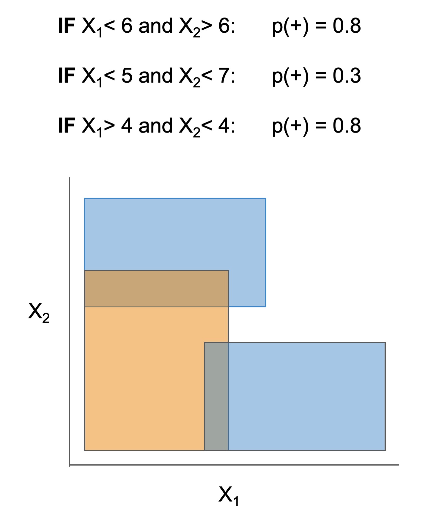
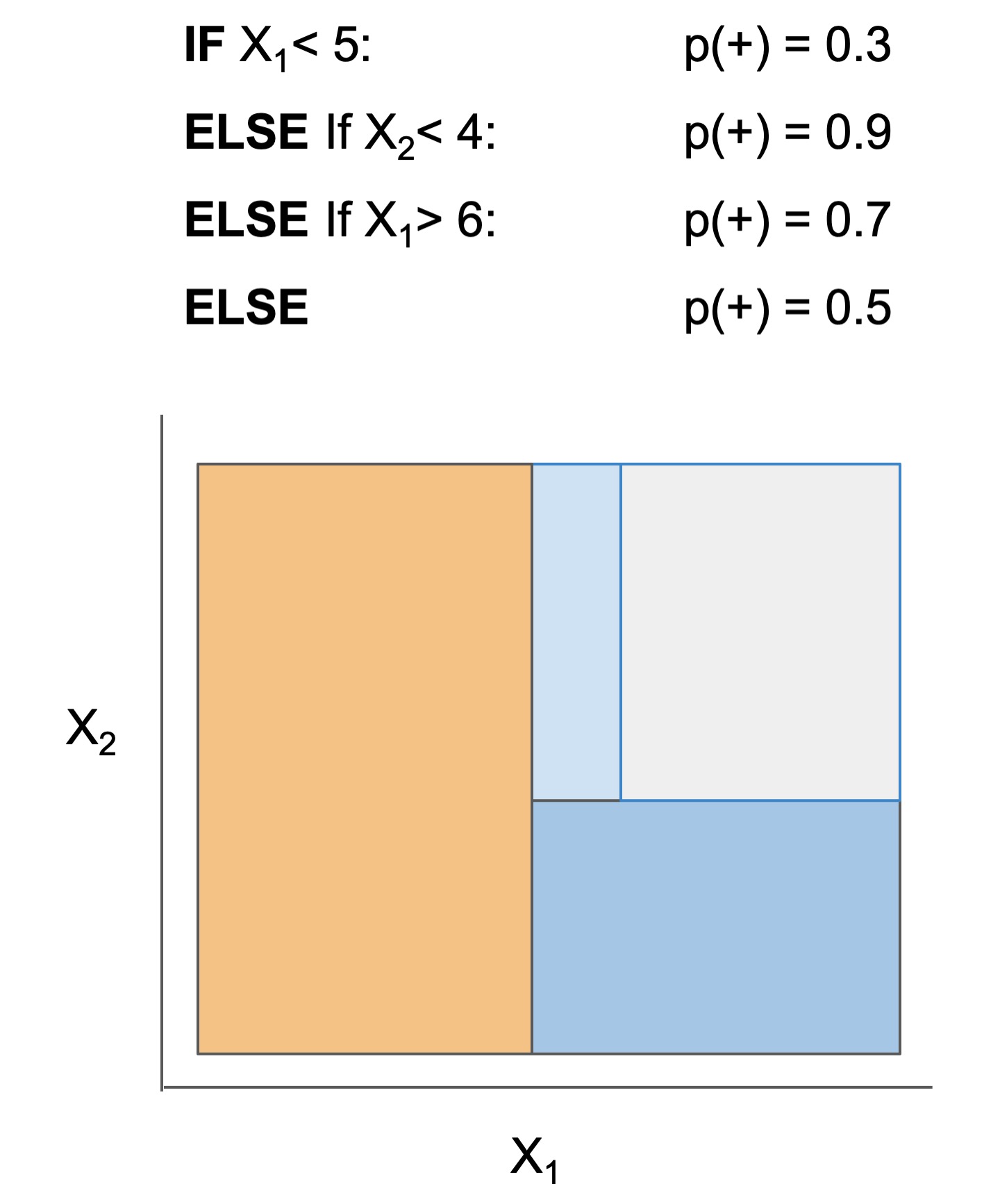
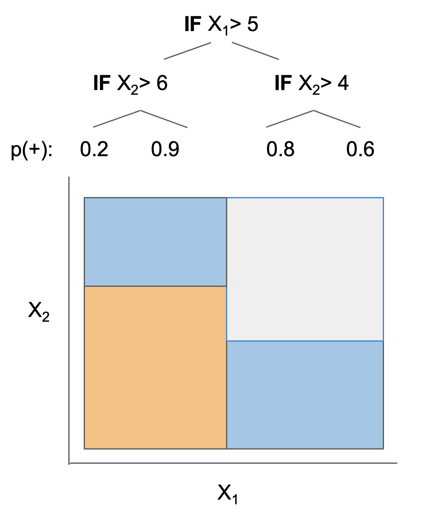
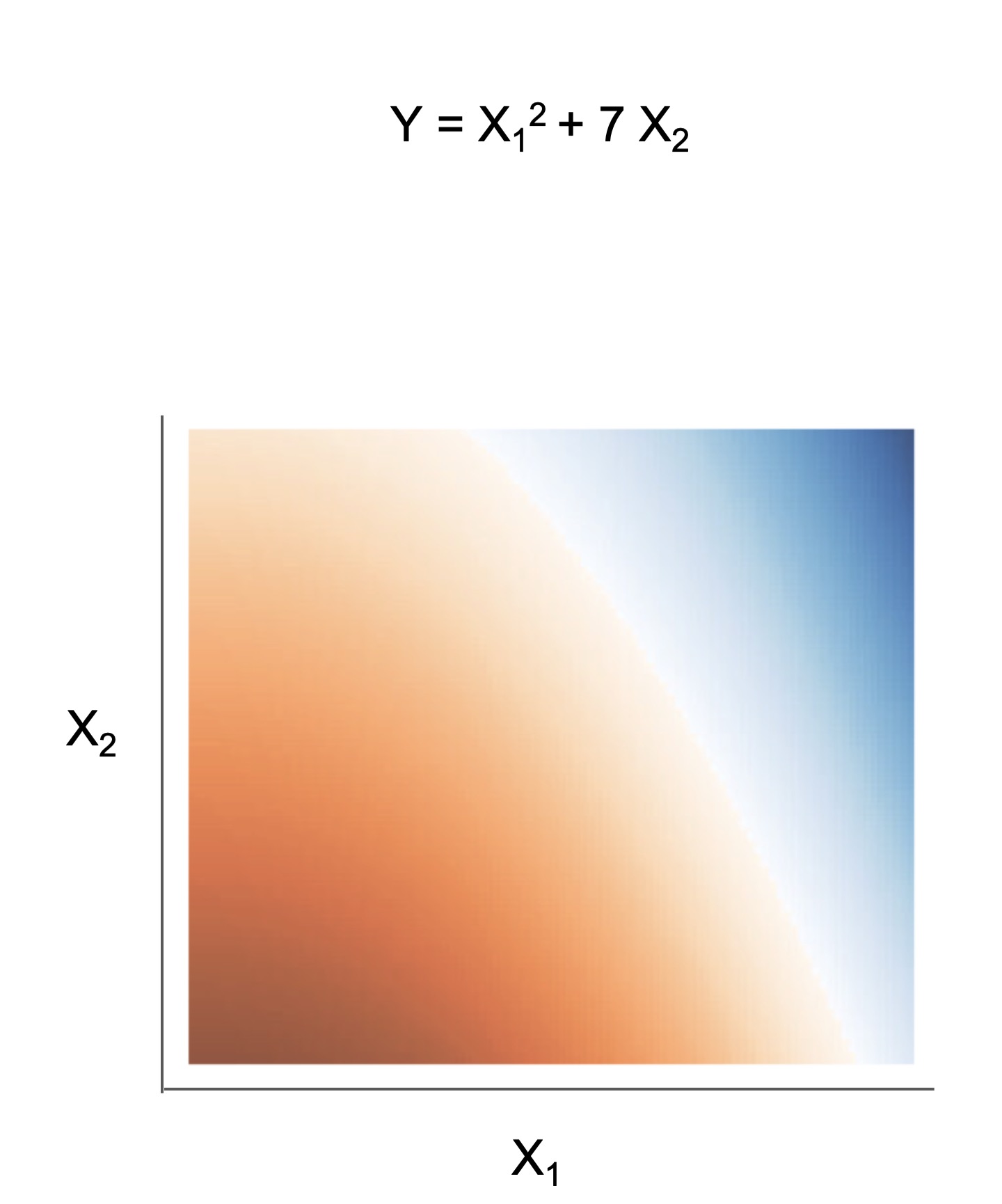
The final form of the above models takes one of the following forms, which aim to be simultaneously simple to understand and highly predictive:
| Rule set | Rule list | Rule tree | Algebraic models |
|---|---|---|---|
 |
 |
 |
 |
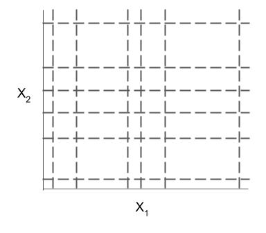
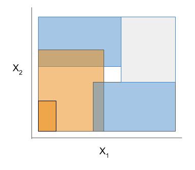
Different models and algorithms vary not only in their final form but also in different choices made during modeling, such as how they generate, select, and postprocess rules:
| Rule candidate generation | Rule selection | Rule postprocessing |
|---|---|---|
 |
 |
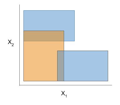 |
Ex. RuleFit vs. SkopeRules
RuleFit and SkopeRules differ only in the way they prune rules: RuleFit uses a linear model whereas SkopeRules heuristically deduplicates rules sharing overlap.Ex. Bayesian rule lists vs. greedy rule lists
Bayesian rule lists and greedy rule lists differ in how they select rules; bayesian rule lists perform a global optimization over possible rule lists while Greedy rule lists pick splits sequentially to maximize a given criterion.Ex. FPSkope vs. SkopeRules
FPSkope and SkopeRules differ only in the way they generate candidate rules: FPSkope uses FPgrowth whereas SkopeRules extracts rules from decision trees.Support for different tasks
Different models support different machine-learning tasks. Current support for different models is given below (each of these models can be imported directly from imodels (e.g. from imodels import RuleFitClassifier):
All of these models follow the standard sklearn estimator API, which is checked for every model in tests/model_api_test.py: fit returns the estimator, predict returns labels drawn from classes_ (strings included), predict_proba returns an (n_samples, n_classes) matrix whose rows sum to 1, DataFrame input sets feature_names_in_,, models can be cloned and configured with get_params/set_params, and every model works inside sklearn pipelines and grid searches.
| Model | Binary classification | Regression | Notes |
|---|---|---|---|
| Rulefit rule set | RuleFitClassifier | RuleFitRegressor | |
| Skope rule set | SkopeRulesClassifier | ||
| FPSkope rule set | FPSkopeClassifier | Like Skope, but generates candidate rules with FPGrowth; requires discretized features | |
| Rulefit rule set (XGBoost) | pass tree_generator=XGBClassifier(...) to RuleFitClassifier |
pass tree_generator=XGBRegressor(...) to RuleFitRegressor |
Requires xgboost |
| FPLasso rule set | FPLassoClassifier | FPLassoRegressor | Lasso over rules mined with FPGrowth; requires discretized features |
| Boosted rule set | BoostedRulesClassifier | BoostedRulesRegressor | |
| SLIPPER rule set | SlipperClassifier | ||
| Bayesian rule set | BayesianRuleSetClassifier | Fails for large problems | |
| Bayesian rule list | BayesianRuleListClassifier | ||
| Greedy rule list | GreedyRuleListClassifier | ||
| OneR rule list | OneRClassifier | ||
| Greedy rule tree (CART) | GreedyTreeClassifier | GreedyTreeRegressor | |
| C4.5 rule tree | C45TreeClassifier | ||
| Optimal rule tree | FastSmallTreeClassifier | Certifiably optimal rather than greedy; needs numba | |
| CCP-pruned rule tree | DecisionTreeCCPClassifier | DecisionTreeCCPRegressor | Prunes a tree to a target complexity via cost-complexity pruning |
| TAO rule tree | TaoTreeClassifier | TaoTreeRegressor | |
| Sparse integer linear model | SLIMClassifier | SLIMRegressor | Requires extra dependencies for speed |
| Tree GAM | TreeGAMClassifier | TreeGAMRegressor | |
| GP GAM | GPGamRegressor | GAM with pairwise interactions; nothing to tune, and deterministic | |
| Greedy tree sums (FIGS) | FIGSClassifier | FIGSRegressor | |
| Hierarchical shrinkage | HSTreeClassifierCV | HSTreeRegressorCV | Wraps any sklearn tree-based model |
| Marginal shrinkage linear model |
MarginalShrinkageLinearModelRegressor | Linear model shrunk towards its marginal effects | |
| BART | BART | Bayesian additive regression trees (slow) | |
| Distillation | DistilledRegressor | Wraps any sklearn-compatible models | |
| AutoML model | AutoInterpretableClassifier️ | AutoInterpretableRegressor️ |
Feature scaling. Most models here work on raw features. SLIMClassifier and
SLIMRegressor are the exception: their coefficients are integers, so features
on very different scales collapse to zero when rounded. Standardize X before
fitting them (they warn if rounding has removed most of the model).
Multiclass. These classifiers handle more than two classes: FIGSClassifier,
GreedyTreeClassifier, HSTreeClassifier, TaoTreeClassifier,
BoostedRulesClassifier, SLIMClassifier, C45TreeClassifier,
DecisionTreeCCPClassifier, FastSmallTreeClassifier and the CV variants. The rule-set and rule-list models are binary-only and raise a
clear error if given a multiclass target, rather than silently treating it as
binary.
Categorical features. FIGS takes them directly — pass the column names and
it one-hot encodes them internally, remembering them for predict:
model = FIGSClassifier().fit(X, y, categorical_features=['pet', 'city'])
model.predict(X)
Other models expect numeric input, so encode categorical columns first (e.g. with
sklearn.preprocessing.OneHotEncoder, or one of the
discretizers for numeric
columns that a rule model needs binarized).
Plotting trees with dtreeviz
Tree-based models can be drawn with dtreeviz.
shadow_tree builds the ShadowDecTree it needs from any imodels tree model:
import dtreeviz
from imodels import FIGSClassifier, shadow_tree

model = FIGSClassifier(max_rules=6).fit(X, y)
viz = dtreeviz.trees.DTreeVizAPI(shadow_tree(model, X, y))
viz.view()
For a model made of several trees (FIGS, boosted rules), pass tree_num to pick
one. Feature and class names default to those the model was fitted with.
dtreeviz is not a dependency and is imported only when this is called.
Inspecting the rules a model learned
Every rule-based model exposes its rules the same way, as a pandas DataFrame with
one row per rule, via get_rules():
from imodels import FIGSClassifier

model = FIGSClassifier(max_rules=4).fit(X_train, y_train, feature_names=feature_names)
model.get_rules()
                                               rule  prediction  tree
0                        FocalNeuroFindings2 <= 0.5       0.117     0
1                         FocalNeuroFindings2 > 0.5       0.427     0
2                             HighriskDiving <= 0.5      -0.008     1
3                              HighriskDiving > 0.5       0.550     1
4  PainNeck2 <= 0.5 and AlteredMentalStatus2 <= 0.5      -0.083     2
5   PainNeck2 <= 0.5 and AlteredMentalStatus2 > 0.5       0.048     2
6                                   PainNeck2 > 0.5       0.058     2
Two columns are always present: rule, the condition as a string, and prediction,
what that rule predicts. Models add their own columns on top — coef, support and
importance for RuleFit, tree for models made of several trees, and weight for
boosted ensembles, which combine their trees by weighted vote. Where a model is
additive, as FIGS is, prediction is that tree's contribution, so the contributions
of the matching rules sum to the model's output.
This works across rule sets, rule lists and tree-based models (RuleFit, SkopeRules,
SLIPPER, greedy and Bayesian rule lists, FIGS, CART, C4.5, TAO, boosted rules, and
hierarchical shrinkage, including the CV variants). It is also available as a
function, imodels.get_rules(model), and takes an optional feature_names argument
to rename the features. Models that aren't rule-based raise a clear error.
Feature importances and leaf assignment
Tree-based models expose feature_importances_ (mean decrease in impurity), the
same measure sklearn's tree models report, so they can be compared directly.
Tree-based models also expose apply(X), which reports which leaf each sample
falls into, using the same node numbering as scikit-learn. A single tree returns
one index per sample; a model made of several trees (FIGS, boosted rules) returns
one column per tree, like RandomForest.apply.
Extras
Data-wrangling functions for working with popular tabular datasets (e.g. compas).
These functions, in conjunction with imodels-data and imodels-experiments, make it simple to download data and run experiments on new models.Explain classification errors with a simple posthoc function.
Fit an interpretable model to explain a previous model's errors (ex. in this notebook📓).Fast and effective discretizers for data preprocessing.
| Discretizer | Reference | Description |
|---|---|---|
| MDLP | 🗂️, 🔗, 📄 | Discretize using entropy minimization heuristic |
| Simple | 🗂️, 🔗 | Simple KBins discretization |
| Random Forest | 🗂️ | Discretize into bins based on random forest split popularity |
Rule-based utils for customizing models
The code here contains many useful and customizable functions for rule-based learning in the util folder. This includes functions / classes for rule deduplication, rule screening, and converting between trees, rulesets, and neural networks.Our favorite methods
After developing and playing with imodels, we developed a few new models to overcome limitations of existing interpretable models.
FIGS: Fast interpretable greedy-tree sums
Fast Interpretable Greedy-Tree Sums (FIGS) is an algorithm for fitting concise rule-based models. Specifically, FIGS generalizes CART to simultaneously grow a flexible number of trees in a summation. The total number of splits across all the trees can be restricted by a pre-specified threshold, keeping the model interpretable. Experiments across a wide array of real-world datasets show that FIGS achieves state-of-the-art prediction performance when restricted to just a few splits (e.g. less than 20).
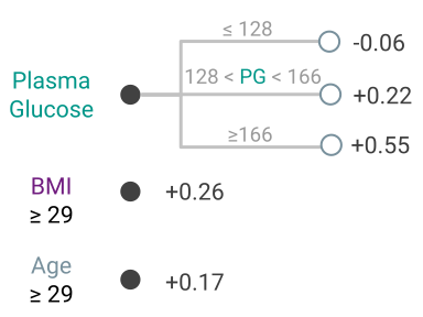
Example FIGS model. FIGS learns a sum of trees with a flexible number of trees; to make its prediction, it sums the result from each tree.
GPGam: additive Gaussian processes over binned features
GPGam fits a generalized additive model with pairwise interactions. Every shape function in it is a Gaussian process over the quantile bins of its feature.
Binning is what makes this practical. Once the features are binned, the exact GP marginal likelihood depends on the data only through the bin co-occurrence counts Z'Z, the bin sums Z'y, and y'y. One pass over the data computes those, and every optimizer step after that costs the same whether the data had a thousand rows or a hundred thousand.
That one likelihood settles every choice a GAM usually leaves to the user. How smooth each shape function should be follows from a mixture of two kernels whose lengthscales are learned and shared across features. Features that explain nothing get amplitudes near zero and drop out, and a hierarchical prior shrinks each kernel's amplitudes toward their centre across features, so that choice is stable across splits. Interactions are screened on the residual; up to 48 are fit jointly, and above a thousand rows the rest, up to five per feature, are backfit on the joint model's residual with each surface's grid resolution picked by comparing likelihoods. Nothing is set by cross-validation and nothing is random, so two fits on the same data give the same model.
from imodels import GPGamRegressor
model = GPGamRegressor().fit(X_train, y_train)

grid, values, std = model.shape_function(0, return_std=True)   # feature 0's curve, with its band
model.kernel_weights(0)                                        # the smooth/rough split the likelihood chose
model.interaction_terms()                                      # the pairs it chose to include
Because the model is a Gaussian process, each curve arrives with a posterior band, so you can see which parts of a shape function the data actually pins down. The post walks through a model fit to California housing, curve by curve and interaction by interaction.
On the development suite (65 datasets, at most 1,000 rows each) GPGam is the strongest interpretable model and second overall to TabPFN. On two held-out suites with every dataset shared with the development suite removed, TabArena and OpenML-CTR23, it is again the strongest interpretable model: first of eleven by mean rank on TabArena and second to TabPFN on CTR23, with a geometric-mean RMSE ratio of 0.97 against explainable boosting machines and wins on 22 of the 35 datasets. Every model in those comparisons was refit on identical preprocessing and the same split.
FastSmallTree: provably optimal small decision trees
FastSmallTree fits the decision tree that minimizes misclassification rate plus a penalty per leaf, over every tree on the binarized features, and certifies that no other tree scores better. This is the objective optimal-tree packages such as GOSDT and STreeD solve. FastSmallTree came out of an autoresearch loop, and most of its speed comes from compiling the whole branch-and-bound search with numba, along with a few tighter bounds, each proved admissible in the post.
from imodels import FastSmallTreeClassifier
model = FastSmallTreeClassifier(regularization=0.05).fit(X_train, y_train)

model.optimal_      # True when the search finished: no other tree on these features scores better
model.objective_    # the proven minimum of error + 0.05 * leaves
model.estimator_    # the tree as an ordinary sklearn DecisionTreeClassifier (plot_tree, dtreeviz, ...)
regularization is the only hyperparameter: larger values give smaller trees. If the time limit is reached first, optimal_ is False and the model warns. The search needs numba (pip install numba); it compiles once per machine, in about 20 seconds, and is cached after that.
On held-out benchmarks built from TabArena, FastSmallTree matches the trees of existing optimal-tree packages while running faster, sometimes by more than 20×, and on the full-size datasets GOSDT and STreeD return no tree for several of them, mostly because they run out of memory. The post has the comparison and the proofs.
Hierarchical shrinkage: post-hoc regularization for tree-based methods
📄 Paper (ICML 2022), 🔗 Post, 📌 Citation
Hierarchical shrinkage is an extremely fast post-hoc regularization method which works on any decision tree (or tree-based ensemble, such as Random Forest). It does not modify the tree structure, and instead regularizes the tree by shrinking the prediction over each node towards the sample means of its ancestors (using a single regularization parameter). Experiments over a wide variety of datasets show that hierarchical shrinkage substantially increases the predictive performance of individual decision trees and decision-tree ensembles.
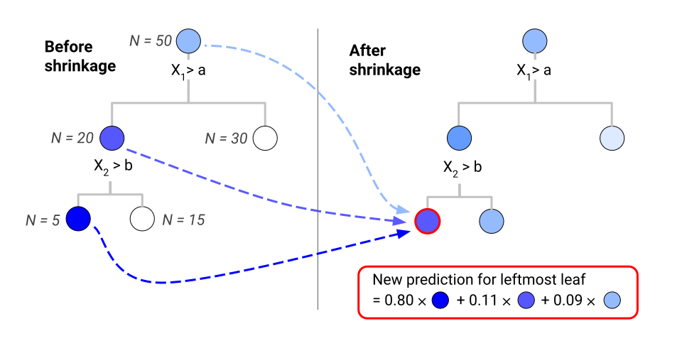
HS Example. HS applies post-hoc regularization to any decision tree by shrinking each node towards its parent.
MDI+: Flexible Tree-Based Feature Importance
MDI+ is a novel feature importance framework, which generalizes the popular mean decrease in impurity (MDI) importance score for random forests. At its core, MDI+ expands upon a recently discovered connection between linear regression and decision trees. In doing so, MDI+ enables practitioners to (1) tailor the feature importance computation to the data/problem structure and (2) incorporate additional features or knowledge to mitigate known biases of decision trees. In both real data case studies and extensive real-data-inspired simulations, MDI+ outperforms commonly used feature importance measures (e.g., MDI, permutation-based scores, and TreeSHAP) by substantional margins.
References
Readings
Reference implementations (also linked above)
The code here heavily derives from the wonderful work of previous projects. We seek to to extract out, unify, and maintain key parts of these projects.- sklearn-expertsys - by @tmadl and @kenben based on original code by Ben Letham
- rulefit - by @christophM
- skope-rules - by the skope-rules team (including @ngoix, @floriangardin, @datajms, Bibi Ndiaye, Ronan Gautier)
- boa - by @wangtongada
Related packages
- gplearn: symbolic regression/classification
- pysr: fast symbolic regression
- pygam: generative additive models
- interpretml: boosting-based gam
- h20 ai: gams + glms (and more)
- optbinning: data discretization / scoring models
- desdeo-brb: distributional rule-based models
Updates
- For updates, star the repo, see this related repo, or follow @csinva_
- Please make sure to give authors of original methods / base implementations appropriate credit!
- Contributing: pull requests very welcome!
Please cite the package if you use it in an academic work :)
@software{
	singh2021imodels,
	title        = {imodels: a python package for fitting interpretable models},
	journal      = {Journal of Open Source Software},
	publisher    = {The Open Journal},
	year         = {2021},
	author       = {Singh, Chandan and Nasseri, Keyan and Tan, Yan Shuo and Tang, Tiffany and Yu, Bin},
	volume       = {6},
	number       = {61},
	pages        = {3192},
	doi          = {10.21105/joss.03192},
	url          = {https://doi.org/10.21105/joss.03192},
}
1 maintainer

Release files for imodels 3.0.2
For a detailed explanation of source distributions (sdists) and built distributions (wheels), please see the package formats documentation.
Source distribution (sdist)
| File | Size | Uploaded | |
|---|---|---|---|
| imodels-3.0.2.tar.gz | 316.7 kB | Details |
Built distribution (wheel)
| File | Interpreter | ABI | Platform | Reset |
|---|---|---|---|---|
| imodels-3.0.2-py3-none-any.whl | Python 3 | none | any | Details |
Total release size: 667.2 kB
Release files / imodels-3.0.2.tar.gz
| Download URL | imodels-3.0.2.tar.gz |
|---|---|
| Size | 316.7 kB |
| Tags | Source |
|
SHA-256 checksum How to use checksums |
f8b3ece9cca0fb90350f0f7776e8f10f5210c7c03293aa716e51473288ded70f
|
|
BLAKE2b-256 checksum How to use checksums |
788029164d658898aa5c794fc96c75a07a0306f98a4a0a50fcf494154d2dfc01
|
| Upload date | |
|
Uploaded using Trusted Publishing? What is trusted publishing? |
No |
| Uploaded via |
uv/0.12.1 {"installer":{"name":"uv","version":"0.12.1","subcommand":["publish"]},"python":null,"implementation":{"name":null,"version":null},"distro":{"name":"macOS","version":null,"id":null,"libc":null},"system":{"name":null,"release":null},"cpu":null,"openssl_version":null,"setuptools_version":null,"rustc_version":null,"ci":null}
|
Release files / imodels-3.0.2-py3-none-any.whl
| Download URL | imodels-3.0.2-py3-none-any.whl |
|---|---|
| Size | 350.4 kB |
| Tags | Python 3 |
|
SHA-256 checksum How to use checksums |
067555d7b210c8872723e4e9e4428fbb3ddbed6daf963ce2f8104d89bdfe5ceb
|
|
BLAKE2b-256 checksum How to use checksums |
671ea0a37a1f804bbb463da101042baaeb25ad86829f8fcf15c788898b4f9dd4
|
| Upload date | |
|
Uploaded using Trusted Publishing? What is trusted publishing? |
No |
| Uploaded via |
uv/0.12.1 {"installer":{"name":"uv","version":"0.12.1","subcommand":["publish"]},"python":null,"implementation":{"name":null,"version":null},"distro":{"name":"macOS","version":null,"id":null,"libc":null},"system":{"name":null,"release":null},"cpu":null,"openssl_version":null,"setuptools_version":null,"rustc_version":null,"ci":null}
|














