Inverse-ODE fitting and sensitivity tools

Project description

🚀 InvODE: Inverse problems on Ordinary Differential Equations


A lightweight, powerful and intuitive Python library for parameter optimization in ordinary differential equation (ODE) systems. invode combines global optimization with local refinement techniques to efficiently find optimal parameter sets for complex dynamical systems.
✨ Features
🎯 Hybrid Optimization Strategy
- Global Exploration: Latin Hypercube Sampling for comprehensive parameter space coverage
- Local Refinement: Gradient-based optimization for precise convergence
- Adaptive Sampling: Progressive search region shrinking for efficient exploration
🔧 Flexible Error Functions
- Built-in metrics: MSE, MAE, RMSE, Chi-squared, Huber Loss
- Regularization: L1, L2, and Elastic Net penalties
- Weighted Fitting: Handle heteroscedastic data with confidence
- Custom Metrics: Easy integration of domain-specific error functions
📊 Advanced Analysis Tools
- Sensitivity Analysis: Identify critical parameters affecting model behavior
- Optimization History: Track convergence and parameter evolution
- Visualization: Built-in plotting for optimization progress and sensitivity
⚡ High Performance
- Parallel Processing: Multi-core evaluation of parameter candidates (to be done!)
- Efficient Sampling: Quasi-Monte Carlo methods for better space filling
- Memory Optimized: Handle large parameter spaces without memory overflow (to be done!)
🛠️ Developer Friendly
- Clean API: Intuitive interface following scikit-learn conventions
- Extensible: Easy to add custom optimization methods and error functions
- Well Documented: Comprehensive documentation with examples and tutorials
🚀 Quick Start
Minimal Example
import numpy as np
from scipy.integrate import odeint
import matplotlib.pyplot as plt
import os
import sys
import scipy.io
from invode import ODEOptimizer, lhs_sample, erf
# Define your ODE system
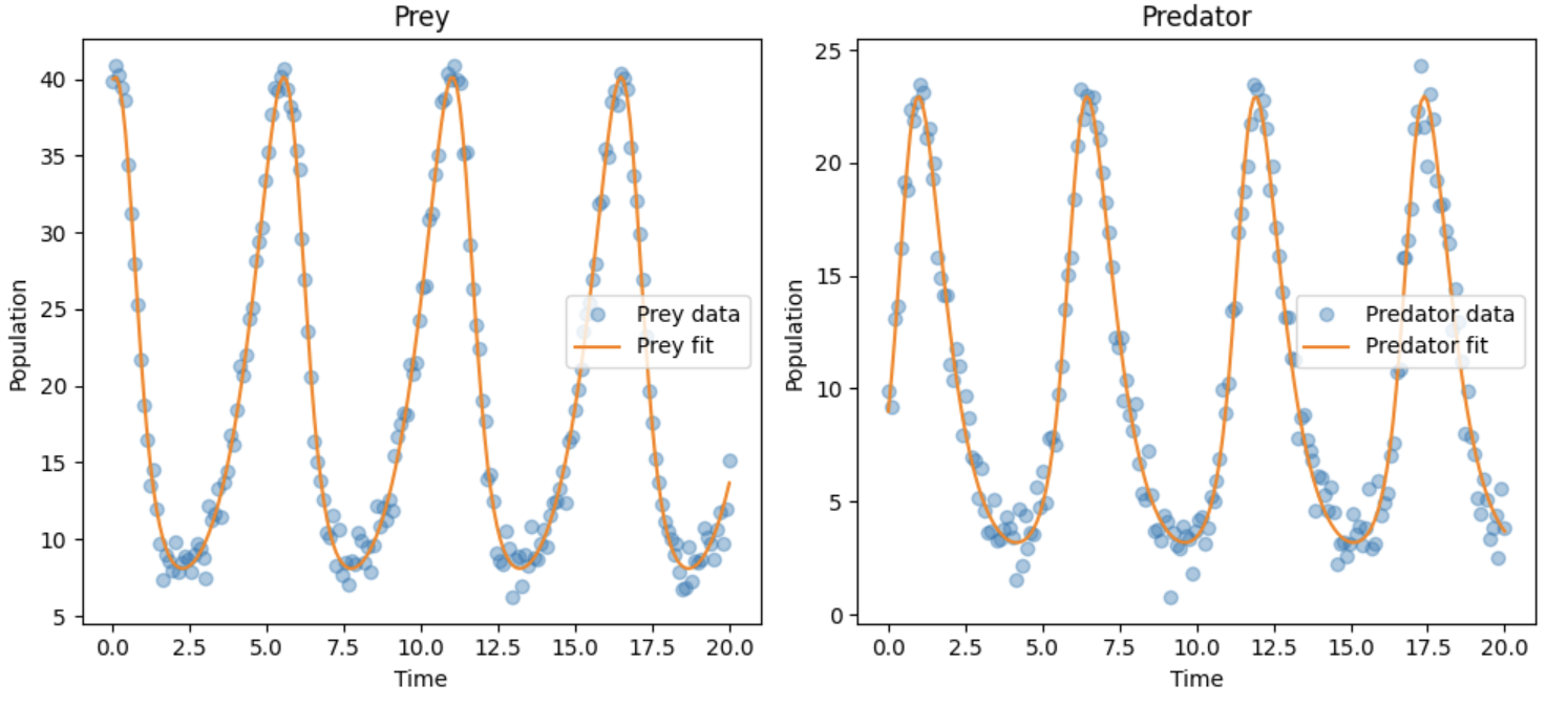
def lotka_volterra(z, t, params):
x, y = z
alpha = params['alpha']
beta = params['beta']
delta = params['delta']
gamma = params['gamma']
dxdt = alpha * x - beta * x * y
dydt = delta * x * y - gamma * y
return [dxdt, dydt]
true_params = {
'alpha': 1.0, # prey growth rate
'beta': 0.1, # predation rate
'delta': 0.075, # predator growth per prey eaten
'gamma': 1.5 # predator death rate
}
t = np.linspace(0, 20, 200)
z0 = [40, 9] # initial population: 40 prey, 9 predators
# Create ODE solver function
def simulate_model(params):
sol = odeint(lotka_volterra, z0, t, args=(params,))
return sol # shape: (N, 2)
# Generate synthetic noisy data (in practice, use your experimental data)
t = np.linspace(0, 20, 200)
z0 = [40, 9] # initial population: 40 prey, 9 predators
true_sol = odeint(lotka_volterra, z0, t, args=(true_params,))
noisy_data = true_sol + np.random.normal(0, 1.0, true_sol.shape)
# Set up optimization
param_bounds = {
'alpha': (0.5, 10),
'beta': (0.05, 0.9),
'delta': (0.05, 0.9),
'gamma': (1.0, 5.0)
}
optimizer = ODEOptimizer(
ode_func=simulate_model,
error_func=mse,
param_bounds=param_bounds,
seed=42,
num_top_candidates=3
)
# Run optimization
optimizer.fit()
best_params, best_error = optimizer.fit()
print(f"Optimal parameters: {best_params}")
print(f"Final error: {best_error:.6f}")
# Analyze parameter sensitivity
from invode import ODESensitivity
sensitivity = ODESensitivity(ode_func=simulate_model,error_func=mse)
sensitivities = sensitivity.analyze_parameter_sensitivity(df)
# Identify most consistently sensitive parameters
summary['mean_abs_sensitivity'] = summary.abs().mean(axis=1)
print(summary.sort_values('mean_abs_sensitivity', ascending=False))
Expected Output
Refining params: {'alpha': 0.5483310416214465, 'beta': 0.068028770810073, 'delta': 0.1451018918331013, 'gamma': 3.1481636450536428}
Refining params: {'alpha': 0.8216385700908369, 'beta': 0.12479204383819222, 'delta': 0.0616377161233344, 'gamma': 1.615577581450748}
Refining params: {'alpha': 1.088028953494527, 'beta': 0.24201471359553078, 'delta': 0.10339353925892915, 'gamma': 1.6535395505316968}
[10]:
({'alpha': 0.9998973552849139,
  'beta': 0.09995621865139477,
  'delta': 0.07482275016126995,
  'gamma': 1.4972199684549248},
 0.9454500024300705)


Optimal parameters: {'alpha': 0.9998973552849139,
 'beta': 0.09995621865139477,
 'delta': 0.07482275016126995,
 'gamma': 1.4972199684549248}

Final error: 0.9454500024300705


correlation  rank_correlation  variance  mutual_info  \
beta      1.000000          1.000000  0.837219     1.000000
alpha     0.939654          0.821020  0.705869     0.890829
delta     0.882231          0.691107  1.000000     0.528090
gamma     0.739286          0.660998  0.000000     0.000000

       mean_abs_sensitivity
beta               0.959305
alpha              0.839343
delta              0.775357
gamma              0.350071
🛠️ Advanced Usage
Custom Error Functions
import invode.erf as erf

# Chi-squared for heteroscedastic data
sigma = np.array([0.1, 0.2, 0.15, 0.3])  # Different uncertainties
error_func = erf.chisquared(data, sigma=sigma)

# Regularized fitting to prevent overfitting
error_func = erf.RegularizedError(data, 'mse', l1_lambda=0.01, l2_lambda=0.1)

# Robust fitting with Huber loss
error_func = erf.huber(data, delta=1.5)
Parallel Optimization (Under dev)
optimizer = invode.ODEOptimizer(
    # ... other parameters
    parallel=True,          # Parallel candidate evaluation
    local_parallel=True,    # Parallel local refinement
    n_samples=100,          # More samples for better parallelization
)
Sensitivity Analysis
# Overall parameter sensitivity
sensitivity = invode.ODESensitivity(ode_func, error_func)
candidates_df = optimizer.get_top_candidates_table()

# Multiple analysis methods
summary = sensitivity.create_sensitivity_summary(
    candidates_df,
    methods=['correlation', 'variance', 'mutual_info']
)

# Evolution over iterations
iteration_sens = sensitivity.analyze_sensitivity_by_iteration(candidates_df)

# Visualize results
fig = sensitivity.plot_sensitivity_analysis(sensitivities)
📄 License
This project is licensed under the MIT License - see the LICENSE file for details.
Why MIT? We believe in open science and want invode to be as widely useful as possible. The MIT license allows both academic and commercial use while maintaining attribution.
🙏 Acknowledgments
- SciPy Community: For providing the foundational numerical computing tools
- Contributors: All the amazing people who have contributed code, documentation, and feedback
- Users: The researchers and engineers who trust invode with their important work
- Academic Partners: Universities and research institutions supporting open source development
Made with ❤️ for the scientific computing community
• 📚 Docs • 🐛 Issues • 💬 Discussions
Release history Release notifications | RSS feed

Download files
Download the file for your platform. If you're not sure which to choose, learn more about installing packages.
Source Distribution
Built Distribution
Filter files by name, interpreter, ABI, and platform.
If you're not sure about the file name format, learn more about wheel file names.
Copy a direct link to the current filters
File details
Details for the file invode-0.1.2.tar.gz.
File metadata
- Download URL: invode-0.1.2.tar.gz
- Upload date:
- Size: 29.5 kB
- Tags: Source
- Uploaded using Trusted Publishing? No
- Uploaded via: twine/6.2.0 CPython/3.11.9
File hashes
| Algorithm | Hash digest | |
|---|---|---|
| SHA256 |
b126a2577639b191a86eb477b9a7d4b717b9291695818dc172550dbd9eaf3254
|
|
| MD5 |
7f663fbeb7b635bc1b64d68bb8fca067
|
|
| BLAKE2b-256 |
009eb481a0371c1782fc644df6f6fc884316a8c59d47e015ec904dac2e0f0c04
|
File details
Details for the file invode-0.1.2-py3-none-any.whl.
File metadata
- Download URL: invode-0.1.2-py3-none-any.whl
- Upload date:
- Size: 33.9 kB
- Tags: Python 3
- Uploaded using Trusted Publishing? No
- Uploaded via: twine/6.2.0 CPython/3.11.9
File hashes
| Algorithm | Hash digest | |
|---|---|---|
| SHA256 |
9b78c58cb5ec774629b72ab41ec13dd852089fc95e6ddf04684d986e50804438
|
|
| MD5 |
2d673017ccd1871160181ca085bb5922
|
|
| BLAKE2b-256 |
c952efc6f7f73709429861e01d8abb26a9e1dcce1a2c69a1f008cc38944817f7
|


