




Inverse Path-Distance Weighted Interpolation
ipdw is a Python package for performing inverse-distance-weighted interpolation using path distances instead of Euclidean distances. In other words, interpolation weights account for domain geometry and obstacles, which is often preferred in geophysical contexts in which "in water" distances are often more relevant to the process at hand than Euclidean distances. For example, this package allows you to quickly and easily interpolate inside a water body, accounting for complex coastlines, islands, and other barriers.
This package is inspired by Stachelek & Madden (2015) and is a Python alternative to the original R package ipdw, although likely using different methodology under the hood. We rely heavily on the fast-marching approach of scikit-fmm to compute path distances, and rely exclusively on matplotlib.path and numpy to make sense of domain geometry information, which can be specified in either raster or vector format. No geospatial packages are required. Due to the use of fast-marching, vectorization, and a reliance on more efficient packages for the compututationally-expensive steps, this package should be quite fast and computationally efficient relative to the complexity of the underlying algorithm.
Installation
Install the latest stable release from PyPi with pip:
pip install ipdw
If you want to install from source, clone this repository, navigate to the new directory, and run python setup.py.
Requirements: numpy, matplotlib, and scikit-fmm
Background
The IPDW estimate for the value $V$ of at some location $(x,y)$ can be written: $$V(x,y) = \frac{ \sum_{i} V_i \cdot d_i^{-P} }{ \sum_{i} d_i^{-P}}$$ for nearest locations $i = [1:N]$, and in which $V_i$ is the input value at location $i$, $d_i$ is the path distance to that location, $P$ is some positive exponent (often 1 or 2), and $N$ is the number of nearest locations to use in the weighting. The weight of each input point decreases for increasing distance away from that point, at a rate of $1/d^P$. If $N=1$, this is equivalent to nearest-neighbor interpolation.
Example Usage
To use this package for interpolation, the user simply needs to provide domain geometry information and the locations/values of input data points. Domain geometry can be specified in one of two ways (i.e. vector or raster format). Regardless of input format, the output will be a raster array.
To specify domain geometry in vector format, the user needs to specify:
- The target
cellsizeof the output array. - The domain
boundary, specified as alistorarrayof $(x,y)$ points for each vertex along the boundary polygon, e.g.[[x1,y1],[x2,y2],...,[xn,yn]]. The length-scale used when specifying these coordinates should be equal to that used for thecellsize. If specified as anarray, dimensions should be(N,2). - Optionally, any internal
holesinside the domain (i.e. obstacles), specified as alistof holes, where each hole has the same input format requirements asboundary.
Then, an example Gridded object can be instantiated as follows:
import ipdw

cellsize = X
boundary = [[x1,y1],[x2,y2],...,[xn,yn]]
holes = [hole_1, hole_2, ..., hole_n]

grid = ipdw.Gridded(cellsize, boundary, holes)
Under the hood, this process creates a binary array of whatever size is needed to span the boundary coordinates at the requested cellsize, and then relies heavily on matplotlib.path.Path to query whether cell locations within that array are (1) inside the domain boundary and (2) not inside one of the specified holes. If a large number of holes are specified, this process may take a while. After the Gridded object has been initialized, the basemap used for interpolation is stored in the grid.raster attribute.
To specify domain geometry in raster format, the user needs to specify:
- A binary
rasterto be used as the basemap for interpolation (in other words, if this raster already exists, we do not need to create it). This raster must be binary (i.e. composed of 1's and 0's), and it will be converted to an integer array during initialization, so anyNaNsshould be set to 0. - The geospatial
extentof thatraster(i.e. the footprint), specified as[xmin, xmax, ymin, ymax].
Then, an example Gridded object can be instantiated as follows (using rasterio as an example way in which one might access a basemap):
import ipdw
import rasterio

src = rasterio.open('path_to_file')
raster = src.read(1).astype(int)
extent = [src.bounds[0], src.bounds[2], src.bounds[1], src.bounds[3]]

grid = ipdw.Gridded(raster=raster, extent=extent)
Note that the combination of either (cellsize, boundary) or (raster, extent) is required to create a Gridded object, they cannot be mixed/matched. Also, if the former pair is specified, the latter will be ignored.
Regardless of which of the two options above was used, performing an interpolation looks the same. The user needs to specify:
input_locationsandinput_valuesfor the data between which we are interpolating- Interpolation settings, most notably
n_nearest(the number of nearest input data points used in the weighting) andpower(the exponent $P$ above), as well as a few other optional parameters described in the function documentation.
Then, it is as simple as:
input_locations = [[x1,y1],[x2,y2],...,[xn,yn]]
input_values = [V1, V2, ..., Vn]

output = grid.interpolate(input_locations, input_values, n_nearest=3, power=1)
in which output is an array with interpolated values in all viable cells, and NaN everywhere else. That's it!
Also, note that there exists another function, Gridded.reinterpolate, which can be used to perform additional interpolations using new input_values from the same locations (and with the same parameter settings), which is faster than re-running interpolate.
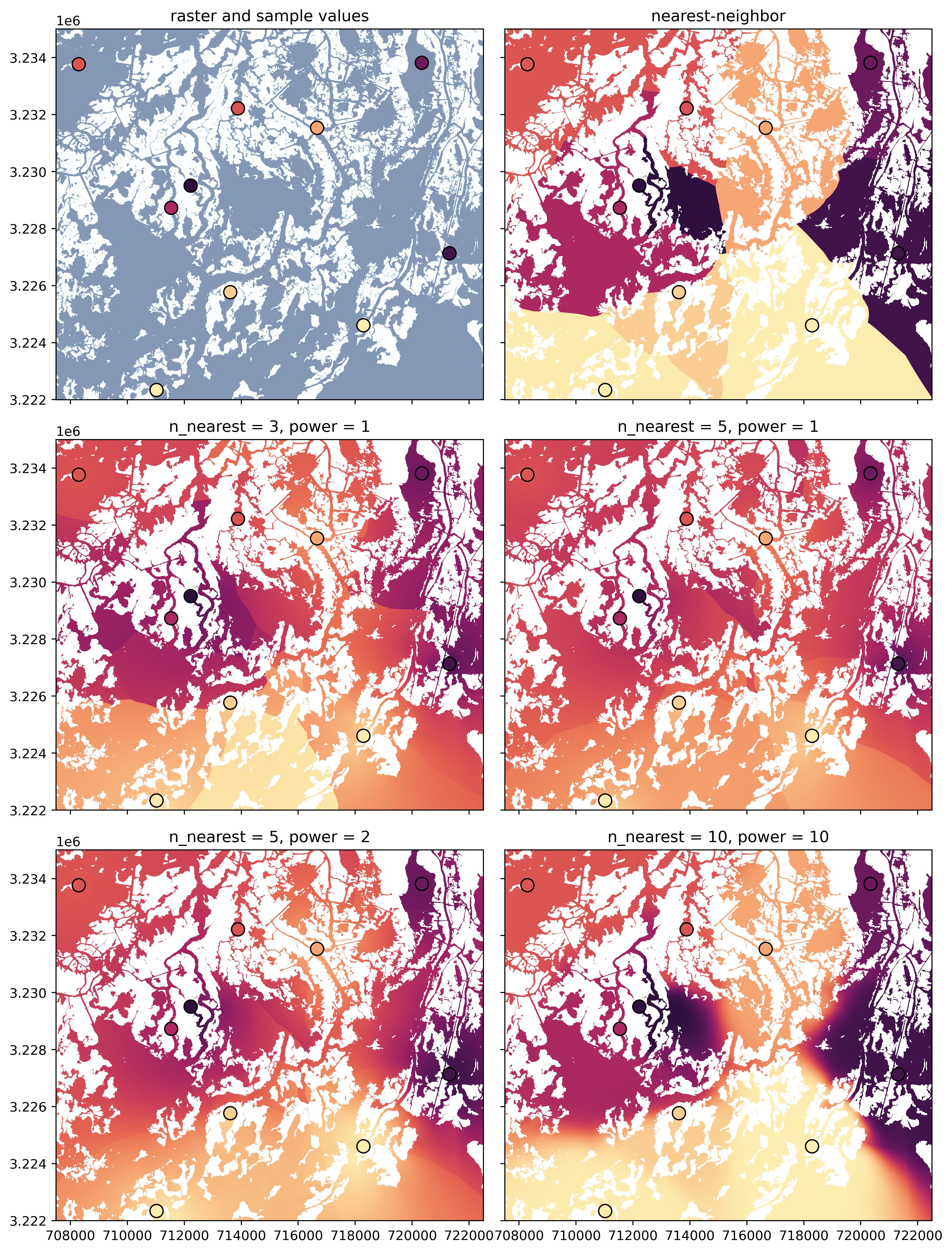
A few example interpolation outputs using different parameter choices are shown below.
Contributing
Please feel free to open an issue or a pull request!
1 maintainer

Metadata
1 maintainer
Release files for ipdw 1.0.1
For a detailed explanation of source distributions (sdists) and built distributions (wheels), please see the package formats documentation.
Source distribution (sdist)
| File | Size | Uploaded | |
|---|---|---|---|
| ipdw-1.0.1.tar.gz | 12.9 kB | Details |
Built distribution (wheel)
| File | Interpreter | ABI | Platform | Reset |
|---|---|---|---|---|
| ipdw-1.0.1-py3-none-any.whl | Python 3 | none | any | Details |
Total release size: 22.6 kB
Release files / ipdw-1.0.1.tar.gz
| Download URL | ipdw-1.0.1.tar.gz |
|---|---|
| Size | 12.9 kB |
| Tags | Source |
|
SHA-256 checksum How to use checksums |
224e8321e0e22807543e920e43e00f5aa073edf701f5ad00d3e93ad394df3282
|
|
BLAKE2b-256 checksum How to use checksums |
f8ac2c5f557ed91656a0c9244df95f4b586d6d107574ebbbc8d30c640b3caafe
|
| Upload date | |
|
Uploaded using Trusted Publishing? What is trusted publishing? |
No |
| Uploaded via |
twine/4.0.2 CPython/3.9.16
|
Release files / ipdw-1.0.1-py3-none-any.whl
| Download URL | ipdw-1.0.1-py3-none-any.whl |
|---|---|
| Size | 9.8 kB |
| Tags | Python 3 |
|
SHA-256 checksum How to use checksums |
9fcc98988b7b179e8e99e8e69c1bd5151db976ad7e3d335c7717fc7a811e1f99
|
|
BLAKE2b-256 checksum How to use checksums |
047cfe8c8525e006bae1cca92d3f9f1f27b9132472d582f347c8d5b3e41fb82d
|
| Upload date | |
|
Uploaded using Trusted Publishing? What is trusted publishing? |
No |
| Uploaded via |
twine/4.0.2 CPython/3.9.16
|














