IWaVE: Image-based Wave Velocimetry Estimation

Project description
IWaVE
Image Wave Velocimetry Estimation
This library performs simultaneous analysis of 2D velocimetry and depth in lakes, coastlines, estuaries and rivers with highly complex bathymetric and wave dynamics through 2D Fourier transform methods using a physics-based approach. Unlike existing velocimetry approaches such as Particle Image Velocimetry or Space-Time Image Velocimetry, the uniqueness of this approach lies in the following:
- velocities that are advective of nature, can be distinguished from other wave forms such as wind waves. This makes the approach particularly useful in estuaries or river stretches affected strongly by wind, or in shallow streams in the presence of standing waves.
- The velocity is estimated based on the physical behavior of the water surface, taking into account the speed of propagation of waves and ripples relative to the main flow. This makes the approach more robust than traditional methods when there are no visible tracers.
- If the depth is not known, it can be estimated along with the optimization of x and y-directional velocity. Depth estimations are reliable only in fast and shallow flows, where wave dynamics are significantly affected by the finite depth.
Gallery
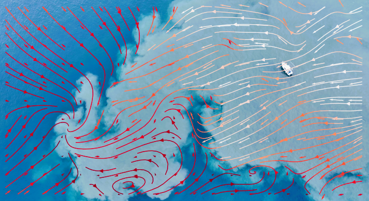
Image license: Creative Commons Attribution 4.0 International (CC BY 4.0). © 2026 Giulio Dolcetti.
This figure gives an example of surface current velocity distribution reconstruction with IWaVE. The video was recorded by a drone on Lake Garda (Italy) during a maintenance opening of the Adige-Garda tunnel. The higher-velocity higher-turbidity plume is caused by the release of water from the Adige River through the 10 km-long tunnel. The background surface velocity distribution outside of the plume is wind-generated.
Purpose
The code is meant to offer an Application Programming Interface (API) for use within more high level applications that utilize the method in conjunction with more high level functionalities such as Graphical User Interfaces, dashboards, or automization routines.
The background and validation of methods are outlined and demonstrated in:
Dolcetti, G., Hortobágyi, B., Perks, M., Tait, S. J. & Dervilis, N. (2022). Using non-contact measurement of water surface dynamics to estimate water discharge. Water Resources Research, 58(9), e2022WR032829. https://doi.org/10.1029/2022WR032829
Examples and prospects of this approach are described in a recent HydroLink article, see https://www.iahr.org/library/infor?pid=40120
The code has been based on the original kOmega Matlab code developed by Giulio Dolcetti (University of Trento, Italy) and released on https://doi.org/10.5281/zenodo.7998891
The API of the code can:
- ingest a set of frames or frames taken from a video
- Slice these into "interrogation window" for which x- and y-directional velocities must be estimated
- Analyze advective velocities per interrogation window using the spectral analysis.
- Additionally estimate the water depth if unknown.
[!NOTE] The sensitivity of water surface dynamics to variations in water depth is minimal. Depth estimations have specific requirements (see below) and can be prone to significant errors. Do not rely on depth estimates for any activity that could pose a risk.
Installation
To install IWaVE, set up a python (virtual) environment and follow the instructions below:
For a direct installation of the latest release, please activate your environment if needed, and type
pip install iwave
If you want to run the examples, you will need some extra dependencies. You can install these with
pip install iwave[extra]
This sets you up with ability to retrieve a sample video, read video frames, and make plots.
Examples
The main functionality is disclosed via an API class IWaVE.
Creating an IWaVE instance
To create an IWaVE instance, you typically start with some settings for deriving analysis windows and
from iwave import Iwave

# Initialize IWaVE object
iw = Iwave(
    resolution=0.01,
    window_size=(64, 64),  # size of interrogation windows over which velocities are estimated
    overlap=(32, 32),  # overlap in space (y, x) used to select windows from images or frames
    time_size=250,  # amount of frames in time used for one spectral analysis
    time_overlap=125,  # amount of overlap in frames, used to establish time slices. Selecting half of
        # time_size implies that you use a 50% overlap in time between frame sets.

)

# print some information about the IWaVE instance
print(iw)
Initializing a IWaVE instance is done by only setting some parameters for the analysis. At this stage we have not loaded any video in memory yet. The inputs have the following meaning:
window_size: the size of so-called "interrogation windows" as a tuple (y, x), i.e. slices of pixels from the original frames that the images are subdivided in. Advective velocities are estimated per interrogation window by fitting a spectral model over space and time within an interrogation window.overlap: overlaps between the interrogation window.(64, 64)here means that an overlap of 50% in both directions is applied.time_size: a spectral model is fitted over several subsets of frames and then averaged. This reduces noise. You can define how large slices are. If you for instance read 300 frames, and use a time_size of 100, 3 subsets of 100 frames are derived, and the spectral model is fitted for all three and then averaged.time_overlap: also for the time, overlap can be used, in the same manner as for spatial overlap usingoverlap.
[!NOTE] Some important remarks on uncertainties: IWaVE employs a spectral approach to compare the observed water surface dynamics with the theoretical expectations for given flow conditions. The key parameters determining the uncertainty of measurements are the spectral resolution, the number of averages, and the sensitivity of surface dynamics to velocity and water depth (see Dolcetti et al., 2022).
- The spectral resolution improves by increasing the window size and/or the time size. Optimal values of
window_sizeshould be similar to the water depth or larger.time_sizeshould be larger than 5 seconds in most applications, ideally around 10 seconds.- The spatial and temporal resolution of the videos (e.g., the pixel size and frame rate) are less critical than the spectral resolution for the accuracy of the estimates. Reasonable results can usually be obtained also with a pixel size of ~5 cm and a frame rate of ~10 fps. Consider downsampling the data if memory or computational time are an issue.
- More averages can significantly improve the convergence of the method. Ideally, one should aim for at least 3 independent slices, regardless of the overlap (e.g., a 30-seconds-long video with a time_size of 10 seconds).
- Short waves are more sensitive to flow velocity, while long waves are more sensitive to water depth. Therefore, a better spatial resolution (smaller pixel size) can improve velocity estimates, while a better spatial resolution (larger window size) can improve the depth estimates. However, only the waves with a wavelength similar or larger than the water depth feel the presence of the bed and can be used to estimate the water depth. Typically, these long waves form naturally in flows with Froude number in the range 0.4 to 1.0. These long waves (wavelength ~ $2\pi F^{2d}$ with $d$ being the depth, must be visible and their wavelength must be smaller than the window size for the depth estimation to be accurate. Otherwise, depth estimates may fail completely due to lack of sensitivity.
Reading in a video
import matplotlib.pyplot as plt
import numpy as np
from matplotlib import patches

from iwave import Iwave, sample_data

iw = Iwave(
    resolution=0.01,  # resolution of videos you will analyze in meters.
    window_size=(64, 64),  # size of interrogation windows over which velocities are estimated
    overlap=(32, 32),  # overlap in space (y, x) used to select windows from images or frames
    time_size=250,  # amount of frames used for one spectral analysis
    time_overlap=125,  # amount of overlap in frames, used to establish time slices. Selecting half of
        # time_size implies that you use a 50% overlap in time between frame sets.
)

# retrieve a sample video from zenodo. This is built-in sample functionality...
fn_video = sample_data.get_sheaf_dataset()
iw.read_video(fn_video, start_frame=0, end_frame=500)

# NOTE: you can also read a list of ordered images with the frames per second set, using iw.read_imgs([...], fps=...)

print(iw)

# show the shape of the read images
print(f"Shape of the available images is {iw.imgs.shape}")

# show the shape of the manipulated windows
print(f"Shape of the available images is {iw.windows.shape}")

# create a new figure with two subplots in one row
f, axs = plt.subplots(nrows=1, ncols=2, figsize=(16, 7))

# plot the first image with a patch at the first window and centers of rest in the first axes instance
first_window = patches.Rectangle((0, 0), 128, 128, linewidth=1, edgecolor='r', facecolor='none', label="first window")
xi, yi = np.meshgrid(iw.x, iw.y)
axs[0].imshow(iw.imgs[0], cmap="Greys_r")
axs[0].add_patch(first_window)
axs[0].plot(xi.flatten(), yi.flatten(), "o", label="centers")
axs[0].legend()
axs[0].set_title("First frame overview")
# plot the first window of the first image in the second axes instance
axs[1].imshow(iw.windows[0][0], cmap="Greys_r")
axs[1].set_title("First frame zoom first window")
plt.show()
You can now see that the IWaVE object shows:
- how many frames are available (if the video is shorter than
start_frameandend_framedictate, you'll get less
frames) - how many time slices are expected from the amount of frames (overlap is included in this)
- The dimensions of the windows
- The y- and x-axis expected from the velocimetry analysis.
You can also see that the frames have actually been read into memory and windowed into a shape that has the following dimensions (in order):
- amount of windows
- amount of frames
- amount of y-pixels per window
- amount of x-pixels per window
Important to note is that the plotted first window on the right is normalized in time by subtracting for each pixel
and time step the temporal mean of that pixel. This is meant to reduce background noise. You may also normalize in
space by passing norm="xy" during the initialization of the IWaVE instance. In this case, the mean of all pixels
in a window is subtracted.
Use iw.read_imgs as suggested in an inline comment to change reading to a set of frames stored as image files.
You then MUST provide frames-per-second explicitly yourself.
Estimating x and y-directional velocity
from iwave import Iwave, sample_data
import matplotlib.pyplot as plt
from matplotlib import patches

# the velocity optimization process is parallelized, for this, you MUST wrap
# your script in a function and protect it with a `if __name__ == "main":` check
def main():
  iw = Iwave(
      # repeat from example above...
  )

  iw.velocimetry(
    alpha=0.85,  # alpha represents the depth-averaged velocity over surface velocity [-]
    depth=0.3,  # depth in [m] has to be known or estimated. If depth = 0, then the depth is estimated.
  )

  ax = plt.axes()
  ax.imshow(iw.imgs[0], cmap="Greys_r")

  # add velocity vectors
  iw.plot_velocimetry(ax=ax, color="b", scale=10)  # you can add kwargs that belong to matplotlib.pyploy.quiver

  # plot the measured spectra and fitted dispersion relation (modify window_idx to visualize different windows)
  fig, axs = plt.subplots(nrows=1, ncols=2, figsize=(15, 7))
  p1 = iw.plot_spectrum_fitted(window_idx=4, dim="x", ax=axs[0])
  axs[0].set_xlim([-100, 100])
  plt.colorbar(p1, ax=axs[0])
  p2 = iw.plot_spectrum_fitted(window_idx=4, dim="y", ax=axs[1])
  axs[1].set_xlim([-100, 100])
  plt.colorbar(p2, ax=axs[1])
  plt.show()

if __name__ == "__main__":
    main()
This estimates velocities in x and y-directions (u, v) per interrogation window and plots it on a background. If the water depth is not supplied, a water depth of $d=1$ m is assumed. With IWaVE, variations in water depth have a small but sometimes non-negligible impact on the velocity calculations. Therefore, it is recommended to set a representative value for depth, even when this is not known accurately.
Optimisation algorithm
The flow parameters are calculated by maximising the cross-correlation between the measured spectrum of the surface elevation and a synthetic spectrum generated according to linear wave theory. This is done using a differential evolution algorithm (scipy.optimize.differential_evolution) which maximises the chances to identify a global maximum but may converge slowly, especially when the window size is large and/or there are more parameters to be estimated (e.g., also the water depth).
pass_downsampling = [2, 1] (default) will run the optimisation in two steps. The first step
employs a trimmed
spectrum with reduced dimensions by a factor of 2, and is used to identify an initial estimate of the flow velocity (depth effects are
neglected during the first step, even when depth==0). During the second step, the search of the optimum is confined
within a region between -0.1 m/s and +0.1 m/s of the initial estimate. The two-steps approach can reduce the computation time
by around 50% for large problems, but could be less robust if the input images are noisy or have a low resolution. In
that case, it is recommended to set pass_downsampling = [1, 1] to avoid an excessive loss in resolution.
[!IMPORTANT] Optimization of the velocities occurs with a possibly large amount of spawned parallelized processes. The
if __name__ == "__main__":construction around the script is necessary to optimize velocities without rerunning the entire script in each spawned subprocess. Like so:import os import iwave def main(): # ... here your core functionalities, making an IWaVE instance, reading video/frames # calling `iw.velocimetry`, storing results, plotting and so on... # at the end, call your function with main functionalities if __name__ == "__main__": main()
[!NOTE] By default, optimizations are parallelized using the maximum amount of CPUs available on your system. If you want to change the amount of CPUs used for optimization, you can set the environment variable
IWAVE_NUM_THREADSto the desired number of CPUs. If you set this environment variable within a python script, you can also set it within the script itself.import os os.environ["IWAVE_NUM_THREADS"] = "1" # make sure you import iwave AFTER setting the environment variable import iwave
Uncertainties
iw.quality is a quality
metric that can represent the confidence in the optimised parameters. The quality $q$ is obtained from the ratio of the
cost functions calculated with the measured spectrum and with the (ideal) synthetic spectrum,
$q = 10 - 2\log_{10}\frac{c_m}{c_i}$, where $c_m$ is the measured cost, and $c_i$ the ideal cost.
Therefore $0 < q < 10$, where 0 is the worst quality and 1 is the best quality. iw.cost is the
measured cost. Acceptable quality may vary depending on window size, frame rate, and velocity and depth magnitude.
Values of $q < 0.7$ are often indicative of poor fitting between measured and ideal spectra, which may indicate
erroneous estimates of velocity. The water depth has a relatively small effect on the cost function, therefore high
values of $q$ are not sufficient indicators of accurate depth estimation, although low values of $q$ are usually
indicative of large uncertainties in both velocity and depth estimations.
iw.status returns a parameter indicating the exit condition. This corresponds to the "success" of the
differential_evolution optimiser. iw.message returns the "message" field.
Estimating water depth as well as x and y-directional velocity
The depth estimation is enabled by setting depth = 0 in iw.velocimetry:
from iwave import Iwave, sample_data
import matplotlib.pyplot as plt
from matplotlib import patches

iw = Iwave(
    # repeat from example above...
)

iw.velocimetry(
  alpha=0.85,  # alpha represents the depth-averaged velocity over surface velocity [-]
  depth=0  # depth in [m] has to be known or estimated. If depth = 0, then the depth is estimated.
)

f, axs = plt.subplots(nrows=1, ncols=3, figsize=(20, 5))
# Plot u against y for all x values
for i in range(iw.results["u"].shape[1]):
    axs[0].plot(iw.y, iw.results["u"][:, i], "o", label=f'x={iw.x[i]}')
axs[0].set_title("u vs y")
axs[0].set_xlabel("y")
axs[0].set_ylabel("u (m/s)")
# Plot v against y for all x values
for i in range(iw.results["v"].shape[1]):
    axs[1].plot(iw.y, iw.results["v"][:, i], "o", label=f'x={iw.x[i]}')
axs[1].set_title("v vs y")
axs[1].set_xlabel("y")
axs[1].set_ylabel("v (m/s)")
# Plot d against y for all x values
for i in range(iw.results["d"].shape[1]):
    axs[2].plot(iw.y, iw.results["d"][:, i], "o", label=f'x={iw.x[i]}')
axs[2].set_title("depth vs y")
axs[2].set_xlabel("y")
axs[2].set_ylabel("depth (m)")
plt.show()
This estimates velocities in x and y-directions (u, v) and water depth (d) per interrogation window and plots the results.
For developers
To install IWaVE from the source code as developer (i.e. you wish to provide contributions to the code), you must checkout the code base with git using an ssh key authentication. for instructions how to set this up, please refer to https://docs.github.com/en/authentication/connecting-to-github-with-ssh/adding-a-new-ssh-key-to-your-github-account
To check out the code and install it, please follow the code below:
git clone git@github.com:DataForWater/IWaVE.git
cd IWaVE
pip install -e .
This will install the code base using symbolic links instead of copies. Any code changes will then immediately be reflected in the installation.
In case you wish to install the code base as developer, and have all dependencies for testing installed as well, you can replace the last line by:
pip install -e .[test]
You can now run the tests by running:
pytest ./tests


Download files
Download the file for your platform. If you're not sure which to choose, learn more about installing packages.
Source Distribution
Built Distribution
Filter files by name, interpreter, ABI, and platform.
If you're not sure about the file name format, learn more about wheel file names.
Copy a direct link to the current filters
File details
Details for the file iwave-0.4.0.tar.gz.
File metadata
- Download URL: iwave-0.4.0.tar.gz
- Upload date:
- Size: 50.2 kB
- Tags: Source
- Uploaded using Trusted Publishing? No
- Uploaded via: twine/6.1.0 CPython/3.13.12
File hashes
| Algorithm | Hash digest | |
|---|---|---|
| SHA256 |
067d01c21dd6c34de93172b5c6bc9372195a75f6194ef3a31cf64ddf5b453acf
|
|
| MD5 |
b3d8b66d0852edb39c1cf6a8f66c5c28
|
|
| BLAKE2b-256 |
dae867ba819959fecbdfbbe992707ed1c7c962ee8a3b38e35a5d1dec7599f94c
|
File details
Details for the file iwave-0.4.0-py3-none-any.whl.
File metadata
- Download URL: iwave-0.4.0-py3-none-any.whl
- Upload date:
- Size: 33.9 kB
- Tags: Python 3
- Uploaded using Trusted Publishing? No
- Uploaded via: twine/6.1.0 CPython/3.13.12
File hashes
| Algorithm | Hash digest | |
|---|---|---|
| SHA256 |
59ae68c9a5e8fdc6fa38cdfcfadbb91b96b034298da7295734c7bd1882c64b58
|
|
| MD5 |
9e60d90a53c4c34e5d2341f9692c49cb
|
|
| BLAKE2b-256 |
74dd86cb9a4c29c27f762dd67e35d61423630f4ca0ed593127b2e508a27c9ccd
|


