
jaxpike
Spiking neural networks in JAX. Fast, functional, and honest about its numbers.



import jax
import jaxpike as jp

key = jax.random.key(0)
k1, k2 = jax.random.split(key)

net = jp.Sequential(
    jp.Dense(784, 512, key=k1),
    jp.LIF(tau=20.0),
    jp.Dense(512, 10, key=k2),
    jp.LIF(tau=20.0, surrogate=jp.ATan()),
)

xs = jax.random.uniform(key, (100, 32, 784))  # (time, batch, features)
spikes, state = jp.unroll(net, xs)
logits = jp.spike_rate(spikes)
Why jaxpike
Spiking networks are recurrent networks with a non-differentiable activation, and the frameworks that train them force a choice. Hand-written CUDA kernels are fast, but you only get the neuron models somebody already wrote a kernel for. Everything written in ordinary PyTorch or JAX lets you define any neuron you like and runs an order of magnitude slower.
jaxpike's claim is that the second path no longer costs an order of magnitude. Writing neurons as ordinary JAX functions, it lands within 1.35× of SpikingJelly's hand-written CuPy kernels and 31–43× ahead of everything else measured — at a fraction of the memory. That is a measured result, not an architectural aspiration; the benchmarks include the configuration where it loses.
Four things get it there:
- Layer-wise execution. Stateless layers are hoisted out of the time loop and evaluated
once across all timesteps, so a
Densebecomes one large matrix multiply instead ofTsmall ones. Bit-identical to walking each timestep, and it is most of the speed. - Three execution strategies behind one signature.
unrollfor sequential BPTT,unroll_checkpointedforO(√T)memory,unroll_parallelforO(log T)depth on reset-free neurons. Interchangeable, and verified to agree. - Memory as a capability, not a footnote. A 256-step BPTT graph fits in 64 MB where SpikingJelly needs 792 MB. On long sequences this stops being a ratio and becomes the difference between a model that runs and one that does not.
- Nothing is registered or subclassed. A neuron is any object with three methods, and a surrogate gradient is one smooth function whose derivative comes from autodiff. There is no supported-model list to fall off.
Plus explicit functional state, so long sequences stream in chunks and truncated BPTT is free; local learning rules — STDP, reward-modulated STDP and Tsodyks–Markram short-term plasticity with the Markram presets — alongside BPTT and e-prop; and NIR import and export, so trained models move to Loihi, SpiNNaker2, Speck and the rest of the neuromorphic ecosystem.
Installation
pip install jaxpike
For a GPU, install JAX for your platform first — see the JAX installation guide:
pip install -U "jax[cuda12]"
pip install jaxpike
From a checkout, with the development and benchmark extras:
uv venv && uv pip install -e ".[dev]"
Requires Python 3.11+.
Documentation
Full documentation, tutorials and API reference are at abdurrezzak.github.io/jaxpike, covering the quickstart, four tutorials — a first network, writing your own neuron, learning without gradients and training on long sequences — a worked SHD training run, a migration guide from snnTorch, why deep SNNs go silent, a model zoo with reproduced results, and a full API reference.
To build the site locally:
cd website && npm install && npm start # Node 20+
Benchmarks
Every framework installed side by side and trained on identical arrays with the same model,
optimizer, loss and dtype, in one container on one NVIDIA T4. SHD, hidden 128, 20 epochs at
batch 256, T=256. Full protocol, ablations and unfavourable results in
benchmarks/README.md.
| framework | training time | peak memory |
|---|---|---|
| SpikingJelly 0.0.0.0.14, multi-step + CuPy | 6.02 s | 792.1 MB |
jaxpike, unroll |
8.12 s | 324.5 MB |
jaxpike, unroll_checkpointed |
11.07 s | 64.2 MB |
jaxpike, unroll_parallel |
15.80 s | 288.1 MB |
| Norse 1.1.0 | 252.21 s | 737.3 MB |
| SpikingJelly, Torch backend | 260.62 s | 696.3 MB |
| snnTorch 1.0.0 | 347.18 s | 675.8 MB |
Accuracy is matched rather than traded away: 0.7532 ± 0.0292 on SHD across five seeds, against the 0.70–0.75 band published for Spyx under the same protocol.
Anything that steps through time in a Python loop is 31–43× slower, which is most of the
field. unroll_checkpointed holds a 256-step BPTT graph in 64 MB where SpikingJelly needs
792 MB. SpikingJelly's fused CuPy kernel remains 1.35× faster than the best jaxpike path
and is not beaten; the gap is entirely in the neuron time loop, where 83% of a training step
is spent.
Core concepts
Defining a neuron
Any module following the state contract works. Nothing is registered, subclassed or special-cased:
init_state(input_shape) -> state pytree
out_shape(input_shape)  -> output shape
__call__(state, x)      -> (new_state, spikes)
Add an optional parallel_apply(state, xs) and the layer becomes eligible for
unroll_parallel.
Defining a surrogate gradient
Write the smooth relaxation. The forward pass emits an exact binary spike and the backward pass differentiates the relaxation, so the two cannot drift apart, and the derivative can be finite-difference tested:
class MySurrogate(jp.Surrogate):
    slope: float = 10.0

    def relaxation(self, v):
        return jax.nn.sigmoid(self.slope * v)
Arbitrary topologies
Sequential is a straight chain. Graph wires any layer to any other — recurrence, skip
connections, branching, fan-in:
net = jp.Graph(
    nodes={
        "w_in": jp.Dense(700, 128, key=k1),
        "hidden": jp.LIF(tau=20.0),
        "w_rec": jp.Dense(128, 128, key=k2),
        "w_out": jp.Dense(128, 20, key=k3),
        "out": jp.LeakyIntegrator(tau=20.0),
    },
    edges=[
        ("input", "w_in"),
        ("w_in", "hidden"),
        ("hidden", "w_rec"),
        ("w_rec", "hidden"),  # closes a cycle
        ("hidden", "w_out"),
        ("w_out", "out"),
    ],
    output="out",
)
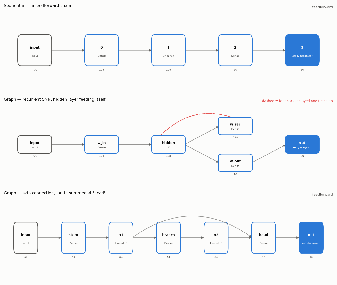
Two rules make any wiring well-defined. A node with several incoming edges sums them,
which is what a synapse does and what makes fan-in and skip connections work without special
syntax. An edge that closes a cycle reads the previous timestep, because a cycle cannot be
resolved within one step — that is what makes a recurrent SNN recurrent, and Graph finds the
back-edges automatically.
A recurrent Graph cannot run parallel-in-time and raises rather than quietly computing
something else.
Spiking convnets
Layout is NHWC — (time, batch, height, width, channels) — because XLA's convolutions are
written for channels-last and NCHW forces a transpose around every operation.
gain = jp.lif_gain(tau=20.0)

net = jp.Sequential(
    jp.Conv2d(2, 32, 3, key=k1, gain=gain),  # 2 channels: DVS on/off events
    jp.LinearLIF(tau=20.0, threshold=0.2),
    jp.Pool2d(2),
    jp.Conv2d(32, 64, 3, key=k2, gain=gain),
    jp.LinearLIF(tau=20.0, threshold=0.2),
    jp.Pool2d(2),
    jp.Flatten(),
    jp.Dense(64 * 8 * 8, 10, key=k3, gain=gain),
    jp.LinearLIF(tau=20.0, threshold=0.2),
)
Convolution and pooling are stateless, so a spiking convnet runs through unroll_parallel
end to end.
Why deep SNNs go silent
Deep spiking networks have a failure mode that ANNs do not: activity decays multiplicatively with depth until nothing reaches the output, and a silent network has no gradient anywhere to recover from. A three-layer spiking convnet with standard LeCun initialization:
| layer 1 | layer 2 | layer 3 | |
|---|---|---|---|
| plain LeCun init | 0.045 | 0.000 | 0.000 |
with gain=lif_gain(tau) |
0.380 | 0.327 | 0.200 |
A LIF membrane is an exponential moving average, which attenuates signal standard deviation by
sqrt((1-a)/(1+a)) — a factor of 6.3 at tau=20. Weights initialized for unit-variance
activations therefore produce membranes six times smaller than intended, sitting below
threshold. jp.lif_gain(tau) returns the compensating factor.
Plasticity
Local learning rules that use no loss function, no gradients and no backward pass. A synapse changes strength from the relative timing of the spikes at its two ends, which is why neuromorphic hardware can implement them directly.
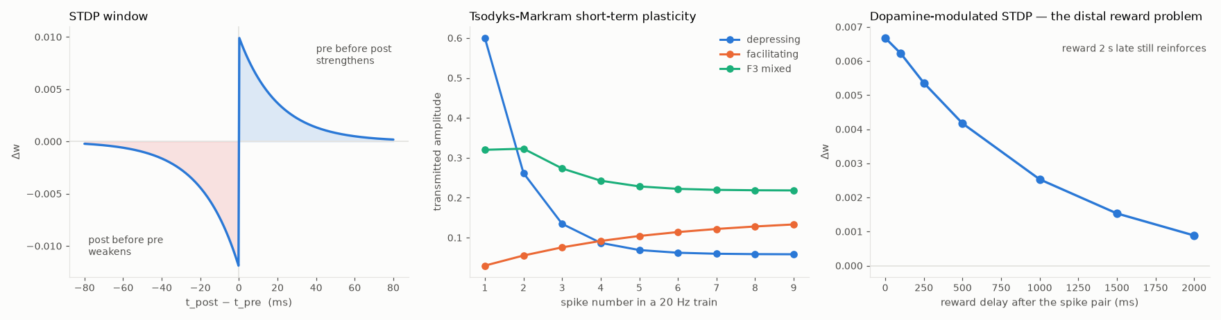
Spike-timing-dependent plasticity. Whole spike trains in, updated weights out:
rule = jp.STDP(tau_pre=20.0, tau_post=20.0)
weight, state = rule(weight, pre_spikes, post_spikes)  # (T, batch, n) trains
jp.stdp_window(delta_t) returns the learning window itself, for plotting or for checking
parameters against a published figure.
Short-term plasticity — depression and facilitation acting on transmission over hundreds of milliseconds without changing the underlying weight. Five presets from the Markram characterization of cortical synapses ship with it:
rule = jp.TsodyksMarkram(*jp.MARKRAM_PRESETS["depressing"])  # or facilitating,
state = rule.init_state(input_shape)  # F1_facilitating,
state, transmitted = rule(state, spikes)  # F2_depressing, F3_mixed
TsodyksMarkram follows the ordinary state contract, so it drops into a Sequential between a
neuron and the layer it drives.
Reward-modulated STDP solves the distal reward problem: a spike pair leaves a slowly
decaying eligibility trace, and the weight only changes when dopamine arrives. With
tau_c = 1000, a reward a full second late still finds the trace alive and credits the right
synapse.
rule = jp.DopamineSTDP(tau_c=1000.0)
weight, state = rule(weight, pre_spikes, post_spikes, reward)
Full details in the plasticity guide and reference.
Visualization
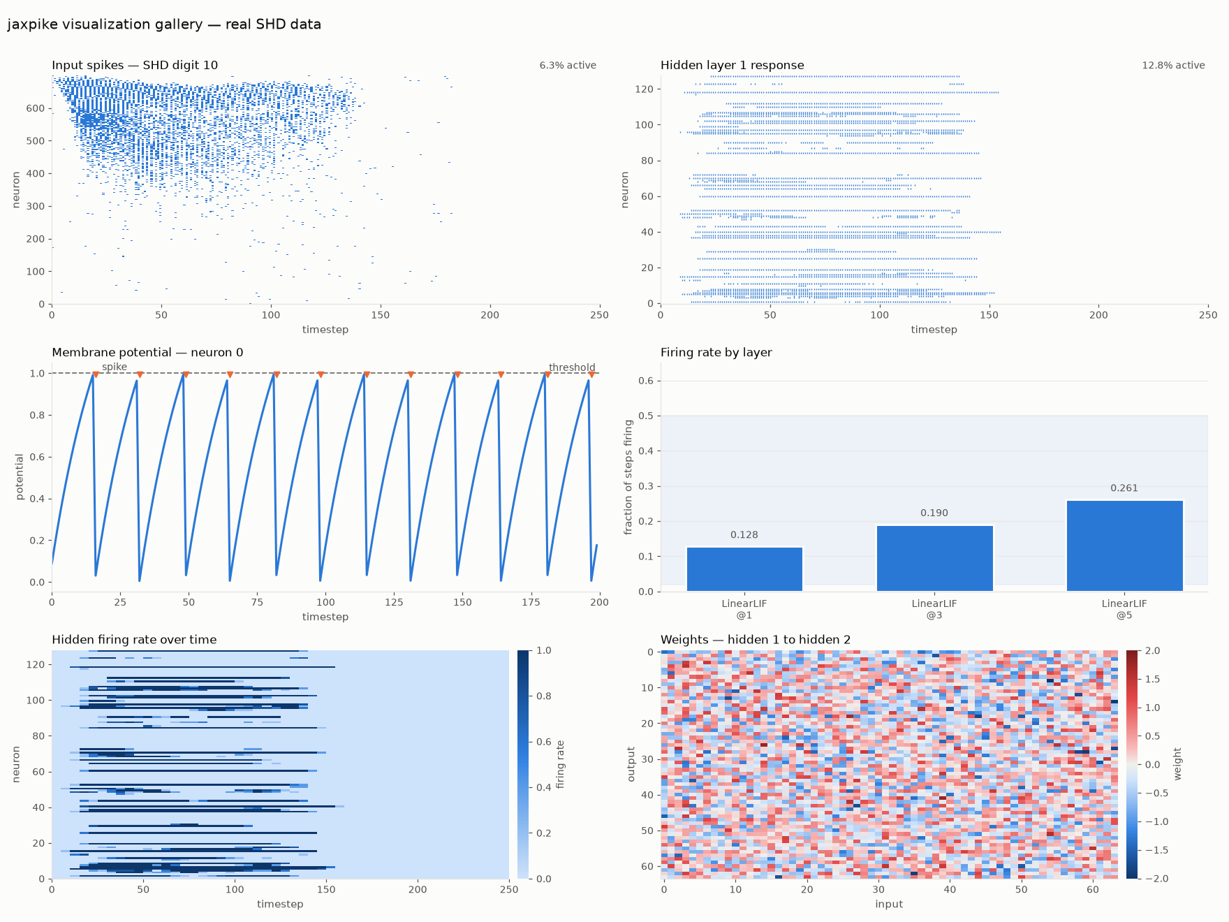
from jaxpike import viz

viz.raster(spikes)
viz.membrane(voltages, spikes=spikes, threshold=1.0)
viz.layer_rates_from(net, xs)  # check for silent or saturated layers
viz.rate_heatmap(spikes)
viz.weights(net.layers[0].weight)
Every function takes an optional ax and returns it, so plots compose into larger figures.
viz.Theme.dark() switches to a dark surface with its own selected colour steps rather than an
inverted light palette.
layer_rates_from is the one to reach for first: it plots the firing rate after every spiking
layer and labels any that have gone silent or saturated.
Hardware export via NIR
NIR is the field's interchange format. Exporting to it lets a model trained here run in snnTorch, Norse, Spyx, Lava, Rockpool or Nengo, and deploy to Intel Loihi, SpiNNaker2, BrainScaleS-2, SynSense Speck or Xylo.
from jaxpike import nir

nir.save(net, "model.nir", input_shape=(1, 700), dt_seconds=1e-3)
net = nir.load("model.nir")
Three things to know, all verified by round-trip tests:
Units are not standardized by NIR. It stores tau in seconds; jaxpike stores it in
timesteps. dt_seconds declares what one timestep physically means, and getting it wrong
rescales every time constant in the model.
Some models cannot be exported, and those raise rather than silently changing.
reset="subtract" has no NIR equivalent, and neither do max pooling, adaptive thresholds,
Izhikevich dynamics or short-term plasticity.
Leaving the library is not bit-exact. NIR specifies a differential equation, not a
discretization — jaxpike solves it exactly, Norse uses forward Euler. snnTorch assumes
dt = 1e-4 s regardless of the file and has no mapping for NIR's LI node. Check numerically
on the far side.
Roadmap
Implemented and benchmarked: the neuron zoo, arbitrary topologies, three execution strategies, surrogate gradients, STDP and short-term plasticity, e-prop, NIR interchange, and visualization.
Not yet built, in priority order:
- Compiled neuron kernels. Tracing a user's neuron to a jaxpr and generating a fused Pallas kernel plus its custom VJP. This is where the remaining 1.35× lives, and it is currently untested rather than unproven: Pallas requires compute capability 8.0 or higher, and the hardware available to this project is sm_75.
- Parallel-in-time for reset neurons. Chunked scan and DEER-style fixed-point iteration,
extending
unroll_parallelbeyond the reset-free case. - Sparse event-driven matmul. Spikes are 1–5% dense; dense compute discards most of that.
- More learning rules. OTTT, SLTT, FPTT and forward-mode alongside BPTT and e-prop.
- Multi-device sharding over batch and time.
Development
uv venv && uv pip install -e ".[dev]"
.venv/bin/pytest
.venv/bin/ruff check . && .venv/bin/ruff format --check .
Benchmarks against other frameworks require an NVIDIA GPU and are run remotely; see
benchmarks/README.md.
Citation
@software{jaxpike,
  title  = {jaxpike: spiking neural networks in JAX},
  author = {Efe, Abdurrezak},
  year   = {2026},
  url    = {https://github.com/abdurrezzak/jaxpike}
}
License
Apache-2.0.
1 maintainer

Download files
Download the file for your platform. If you're not sure which to choose, learn more about installing packages.
Source Distribution
Built Distribution
Filter files by name, interpreter, ABI, and platform.
If you're not sure about the file name format, learn more about wheel file names.
Copy a direct link to the current filters
File details
Details for the file jaxpike-0.1.4.tar.gz.
File metadata
- Download URL: jaxpike-0.1.4.tar.gz
- Upload date:
- Size: 78.9 kB
- Tags: Source
- Uploaded using Trusted Publishing? Yes
- Uploaded via:
twine/7.0.0 CPython/3.13.14
File hashes
| Algorithm | Hash digest | |
|---|---|---|
| SHA256 |
4d91886663a1898dc33cd0ed75f4d6c20d2663d62ed765a57b05a073ec8d726a
|
|
| MD5 |
3bb966de6c9a29df771980d19e2c8ac7
|
|
| BLAKE2b-256 |
d81b0ad893ff64790bbb8c5a3c5db992c47507e8b408a85c4773b5ab4103dbb8
|
Provenance
The following attestation bundles were made for jaxpike-0.1.4.tar.gz:
Publisher:
release.yml on abdurrezzak/jaxpike
-
Statement:
-
Statement type:
https://in-toto.io/Statement/v1 -
Predicate type:
https://docs.pypi.org/attestations/publish/v1 -
Subject name:
jaxpike-0.1.4.tar.gz -
Subject digest:
4d91886663a1898dc33cd0ed75f4d6c20d2663d62ed765a57b05a073ec8d726a - Sigstore transparency entry: 2412415012
- Sigstore integration time:
-
Permalink:
abdurrezzak/jaxpike@67403d0fd29ed2051b29cab4986623353d496f7a -
Branch / Tag:
refs/tags/v0.1.4 - Owner: https://github.com/abdurrezzak
-
Access:
public
-
Token Issuer:
https://token.actions.githubusercontent.com -
Runner Environment:
github-hosted -
Publication workflow:
release.yml@67403d0fd29ed2051b29cab4986623353d496f7a -
Trigger Event:
release
-
Statement type:
File details
Details for the file jaxpike-0.1.4-py3-none-any.whl.
File metadata
- Download URL: jaxpike-0.1.4-py3-none-any.whl
- Upload date:
- Size: 54.0 kB
- Tags: Python 3
- Uploaded using Trusted Publishing? Yes
- Uploaded via:
twine/7.0.0 CPython/3.13.14
File hashes
| Algorithm | Hash digest | |
|---|---|---|
| SHA256 |
119f93662ba7e9287e15e2bbfe1c75f4b461ab2556894503258e58297be156f8
|
|
| MD5 |
a41ef119a3717b4d23b2c903f4ac0c1b
|
|
| BLAKE2b-256 |
8f736088e825c2fb894fab9e7e4ec284fcff205c544a269ff9a8cdc45a4ea308
|
Provenance
The following attestation bundles were made for jaxpike-0.1.4-py3-none-any.whl:
Publisher:
release.yml on abdurrezzak/jaxpike
-
Statement:
-
Statement type:
https://in-toto.io/Statement/v1 -
Predicate type:
https://docs.pypi.org/attestations/publish/v1 -
Subject name:
jaxpike-0.1.4-py3-none-any.whl -
Subject digest:
119f93662ba7e9287e15e2bbfe1c75f4b461ab2556894503258e58297be156f8 - Sigstore transparency entry: 2412415130
- Sigstore integration time:
-
Permalink:
abdurrezzak/jaxpike@67403d0fd29ed2051b29cab4986623353d496f7a -
Branch / Tag:
refs/tags/v0.1.4 - Owner: https://github.com/abdurrezzak
-
Access:
public
-
Token Issuer:
https://token.actions.githubusercontent.com -
Runner Environment:
github-hosted -
Publication workflow:
release.yml@67403d0fd29ed2051b29cab4986623353d496f7a -
Trigger Event:
release
-
Statement type:














