
JDtI – Python library for scRNAseq/RNAseq data analysis




Author: Jakub Kubiś
Polish Academy of Sciences
Laboratory of Single Cell Analyses
Description
JDtI enables basic quality control steps such as control of cells per cluster, number of genes per cell, and more advanced tasks like subclustering, integration, and wide visualization. In this approach, we do not drop the cell information during separate set analyses; instead, we use previous cluster cell lineage information for integrating data based on cluster markers and data harmonization. After integration, it is possible to visualize cell interactions and correlations in many ways, including cell distance, correlations, and more.
Despite this, it is also able to conduct DEG analysis between sets, selected cells, or grouped cells, and visualize the results on UMAP, volcano plots, and regression plots comparing pairs of cells. It is very powerful for more advanced analyses focusing on specific issues within the data that may not be discovered in basic analyses.
Additionally, JDtI offers many functions for data visualization and processing within clean visual outputs, such as volcano plots, gene expression analysis of different data types, clustering, heatmaps, and more.

It is compatible with various sequencing approaches, including scRNA-seq and bulk RNA-seq, and supports interoperability with tools such as Seurat, Scanpy, and other bioinformatics frameworks using the 10x sparse matrix format as input. More details about the available functions can be found in the Documentation and Example Usage section on GitHub.
📚 Table of Contents
- Installation
- Documentation
- Example usage
- 1. Basic functions
- 2. Data clustering
- 2.1. Loading class and helper function
- 2.2. Loading data
- 2.3. Initialize Clustering class
- 2.4. Performing PCA
- 2.5. Knee plot of PC
- 2.6. Harmonize data (Harmony)
- 2.7. Find clusters on PC
- 2.8. Perform UMAP
- 2.9. Knee plot of UMAP
- 2.10. Find clusters on UMAP
- 2.11. Visualization of names on UMAP reduced space
- 2.12. Visualization of feature level on UMAP reduced space
- 3. Data integration
- 4. Data subclustering
- 4.1. Loading class
- 4.2. Initialize COMPsc class
- 4.3. Loading data
- 4.4. Select cluster and features for subclustering
- 4.5. Prepare subclustering
- 4.6. Define subclusters
- 4.7. Visualize subclusters features
- 4.8. Adjust subclusters and check features
- 4.9. Calculate DEG for subclusters and visualize
- 4.10. Confirm subclusters and associate with data
Installation
pip install jdti
Documentation
Documentation for classes and functions is available here 👉 Documentation 📄
Example usage
1. Basic functions
1.1. Loading functions
from jdti import *
1.2. Loading data
# load sparse matrix as pd.DataFrame data with creating metadata
data, metadata = load_sparse(path = 'data/set1', name = 'set1')

#load data frame from different data type (.tsv, .txt, .tsv)
data = pd.read_csv('example_data.csv')

# load data from .h5 or other data types and transform to pandas data frame
- Data [features (eg. genes) x sample (eg. cells)]
- Metadata [columns['cell_names', 'sets']]:
- cell_names – sample names corresponding to the columns of Data
- sets – the assignment of each sample to a given dataset, aligned with Data
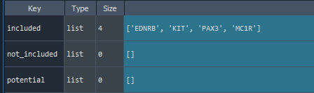
1.3. Features finding
features = find_features(data, features =['KIT', 'MC1', 'EDNRB', 'PAX3'])
- Not found the MC1 feature name, so the potential names are provided

features = find_features(data, features =['KIT', 'MC1R', 'EDNRB', 'PAX3'])
- All feature names have been found
1.4. Names finding
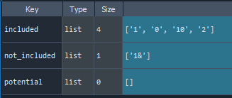
names = find_names(data, names = ['0', '1', '2','10', '1&'])
- As same as in case of 'Features finding'
1.5. Data reducing
# data reducing on found features and names

data_reduced = reduce_data(data,
                features = features['included'],
                names = names['included'])
- return data with selected features & names
1.6. Data averaging and occurrence counting
avg_reduced = average(data_reduced)
occ_reduced = occurrence(data_reduced)
- returns the average or occurrence values computed across all columns that share the same name
1.7. Difference counting (DEG) and visualization
# creating group dict for compare samples
compare_dict = {'g1':['0', '1'],
                'g2':['2','10']}


deg_df = calc_DEG(data,
             metadata_list  = None,
             entities = compare_dict,
             sets = None,
             min_exp = 0,
             min_pct = 0.1,
             n_proc =10)

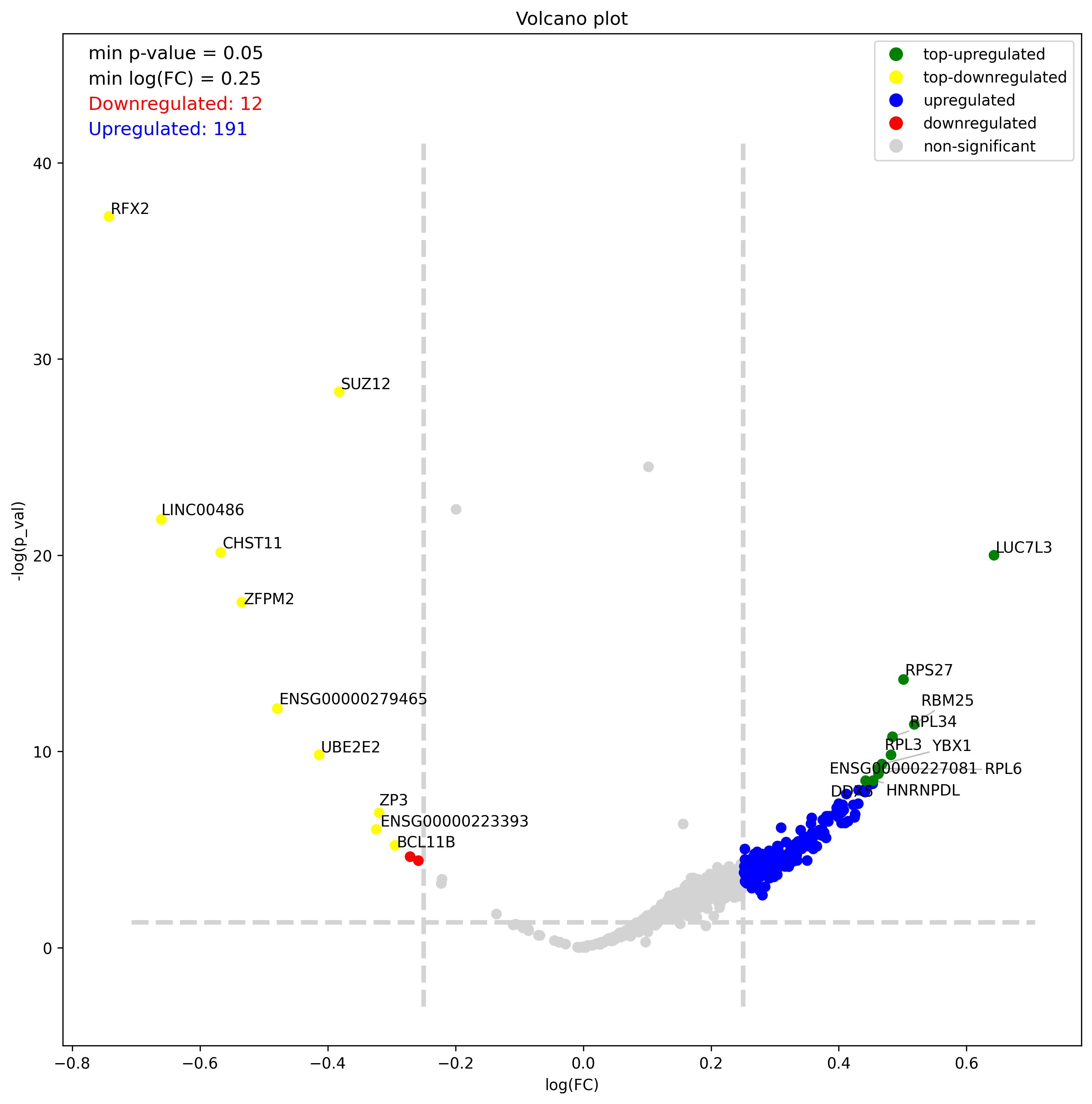
# DEG visualization with volcano plot
fig = volcano_plot(deg_df,
                 p_adj = True,
                 top = 25,
                 p_val = 0.05,
                 lfc = 0.25,
                 standard_scale = False,
                 rescale_adj = True,
                 image_width = 12,
                 image_high = 12)

fig.savefig('volcano.jpeg', dpi=300, bbox_inches='tight')
- DEG data:
feature– Name of the studied featurep_val– P-value (Mann–Whitney) for the studied feature comparing thevalid_groupto all other groups in the analysispct_valid– Percentage of positive (>0) values for the studied feature in thevalid_group*pct_ctrl– Percentage of positive (>0) values for the studied feature in all other groupsavg_valid– Average value of the studied feature in thevalid_groupavg_ctrl– Average value of the studied feature in the remaining groupssd_valid– Standard deviation of the studied feature in thevalid_group*sd_ctrl– Standard deviation of the studied feature in the remaining groupsesm– Cohen’s d effect size metricvalid_group– Name of the sample or group belonging to thevalid_groupadj_pval– Benjamini–Hochberg adjusted p-valueFC– Fold change between the averagedvalid_groupsamples and the averaged remaining sampleslog(FC)– Log₂-transformed fold changenorm_diff– Direct difference between the averagedvalid_groupvalue and the averaged value of the remaining groups
- Volcano plot – Visualization of differentially expressed genes (DEGs) between two groups
1.8. Features visualization
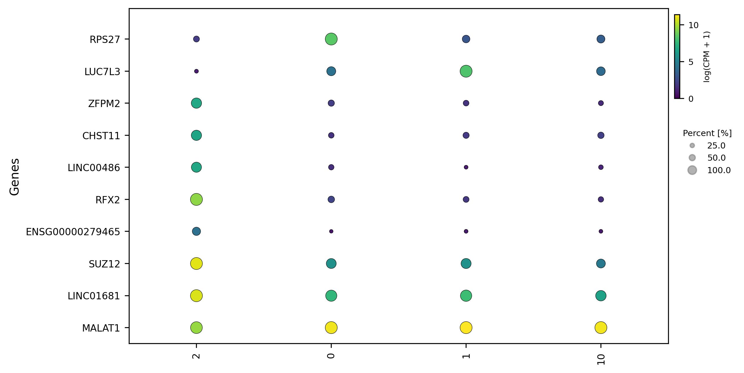
top_10 = deg_df.sort_values(
    ['p_val', 'esm', 'log(FC)'],
    ascending=[True, False, False]).head(10)

data_dot = reduce_data(data,
                features = list(set(top_10['feature'])),
                names = names['included'])


avg = average(data_dot)
occ = occurrence(data_dot)


fig = features_dot(expression_data = avg,
                     occurence_data = occ,
                     features = None,
                     metadata_list = None,
                     colors = 'viridis',
                     hclust = 'complete',
                     img_width = 8,
                     img_high = 5,
                     label_size = 10,
                     size_scale = 100,
                     y_lab = 'Genes',
                     legend_lab = 'log(CPM + 1)',
                     bbox_to_anchor_scale = 25,
                     bbox_to_anchor_perc=(0.91, 0.55),
                     bbox_to_anchor_group=(1.01, 0.4))

fig.savefig('dot.jpeg', dpi=300, bbox_inches='tight')
- Dot plot – Displays expression relationships of DEGs across groups or individual samples
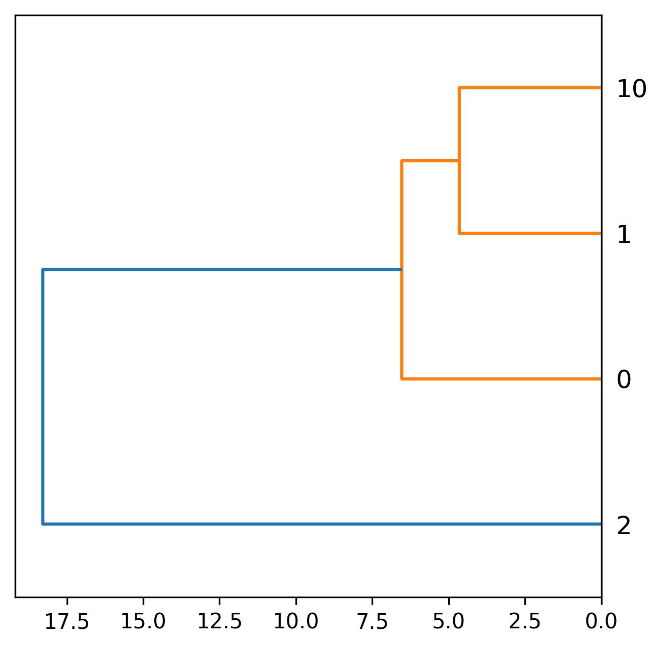
1.9. Relation visualization
fig = development_clust(data = avg,
                      method = 'ward',
                      img_width = 5,
                      img_high = 5)

fig.savefig('development.jpeg', dpi=300, bbox_inches='tight')
- Development plot – A dendrogram showing sample similarity based on the expression features generated using hierarchical clustering
2. Data clustering
2.1. Loading class and helper functions
from jdti import Clustering, load_sparse
2.2. Loading data
# load sparse matrix as pd.DataFrame data with creating metadata
data, metadata = load_sparse(path = 'set1', name = 'set1')

#load data frame from different data type (.tsv, .txt, .tsv)
data = pd.read_csv('example_data.csv')

# load data from .h5 or other data types and transform to pandas data frame
- Data [features (eg. genes) x sample (eg. cells)]
- Metadata [columns['cell_names', 'sets']]:
- cell_names – sample names corresponding to the columns of Data
- sets – the assignment of each sample to a given dataset, aligned with Data
2.3. Initialize Clustering class
clusters = Clustering.add_data_frame(data, metadata)

# attributes with inputed data and metadata
clusters.clustering_data
clusters.clustering_metadata
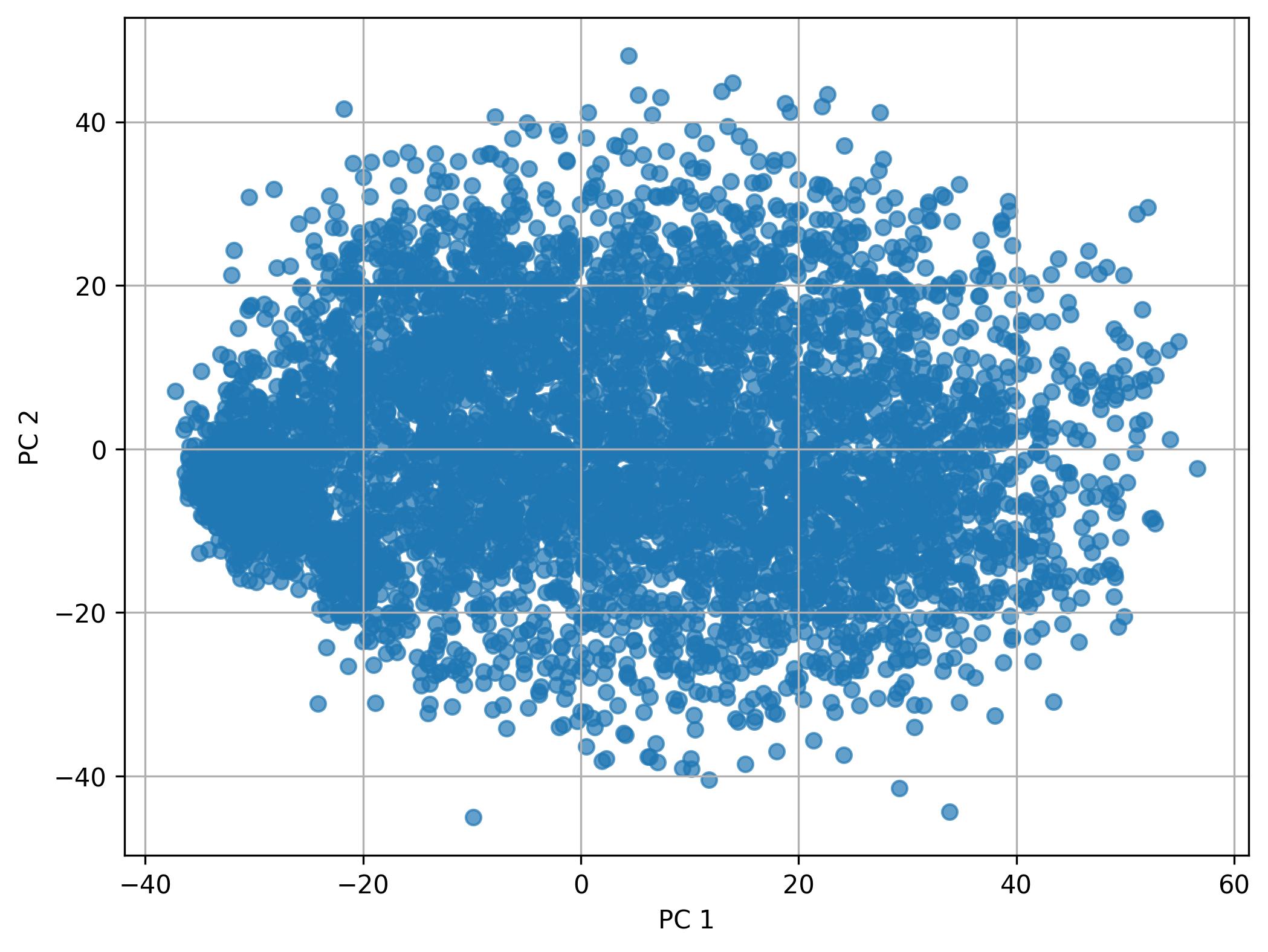
2.4. Performing PCA
fig1 = clusters.perform_PCA(pc_num=50, width=8, height=6)

fig1.savefig('clus_PCA.jpeg', dpi=300, bbox_inches='tight')
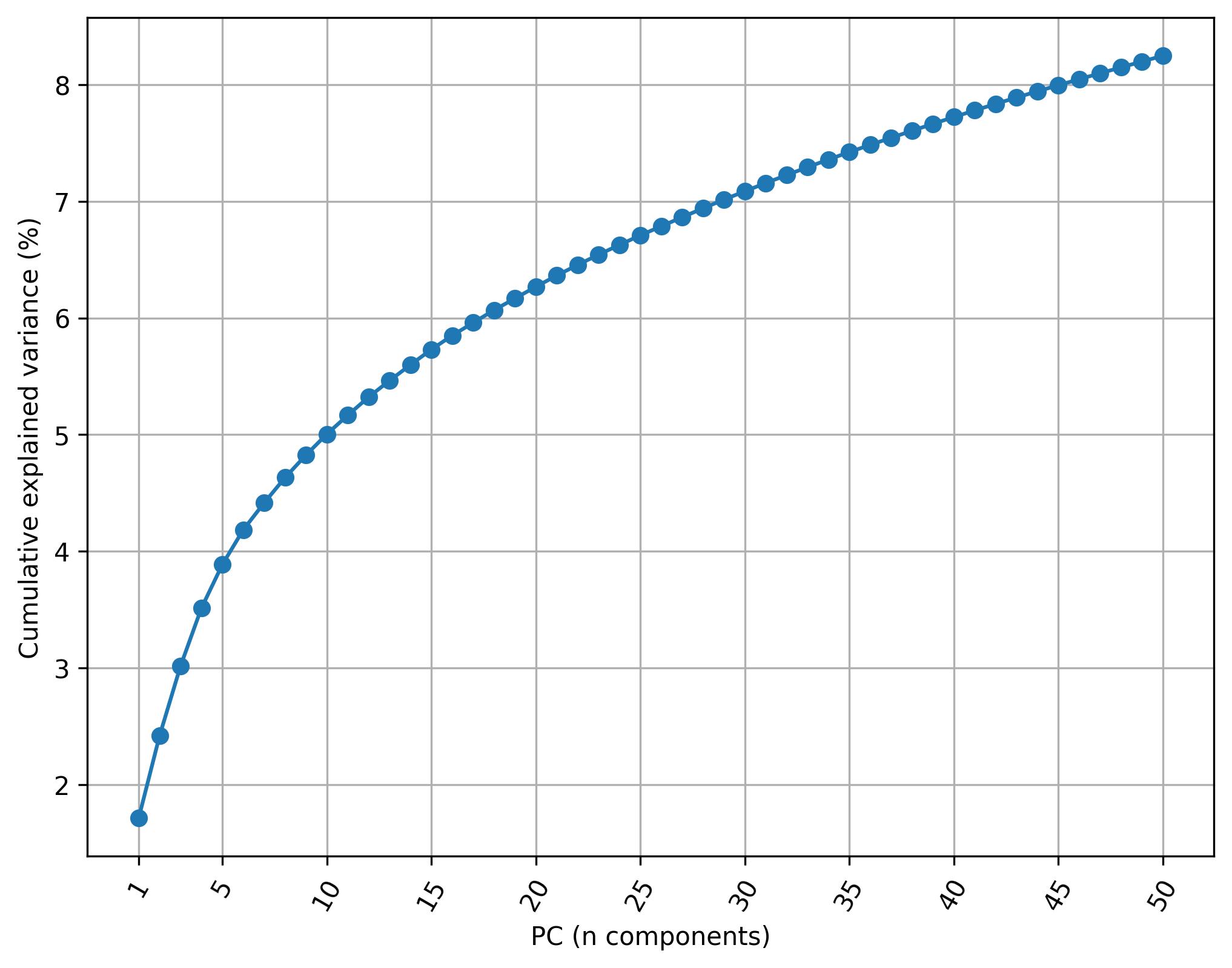
2.5. Knee plot of PC
fig2 = clusters.knee_plot_PCA(width=8, height=6)

fig2.savefig('clus_PCA_knee.jpeg', dpi=300, bbox_inches='tight')
2.6. Harmonize data (Harmony)
# if more than one dataset (provided in metadata) harmonization process can be used
clusters.harmonize_sets()
2.7. Find clusters on PC
fig3 = clusters.find_clusters_PCA(pc_num=50, eps=0.5, min_samples=10, width=8, height=6, harmonized=False)

clusters.return_clusters(clusters='pca')

fig3.savefig('clus_PCA_clusters.jpeg', dpi=300, bbox_inches='tight')
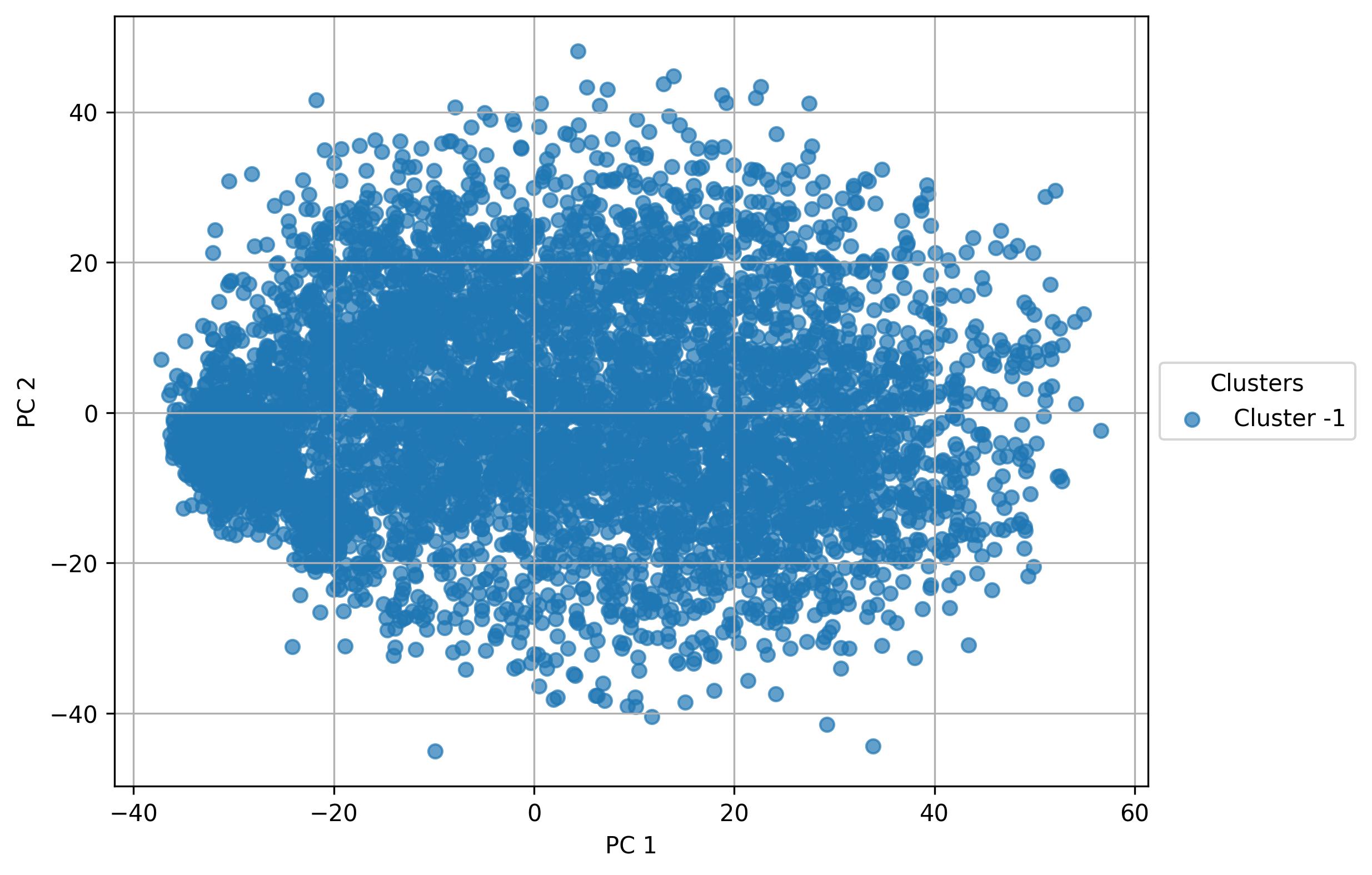
- No cluster detected in linear reduced space
2.8. Perform UMAP
clusters.perform_UMAP(factorize=True, umap_num=50, pc_num=5, harmonized=False)
2.9. Knee plot of UMAP
fig4 = clusters.knee_plot_umap(eps=0.5, min_samples=10)

fig4.savefig('clus_UMAP_knee.jpeg', dpi=300, bbox_inches='tight')
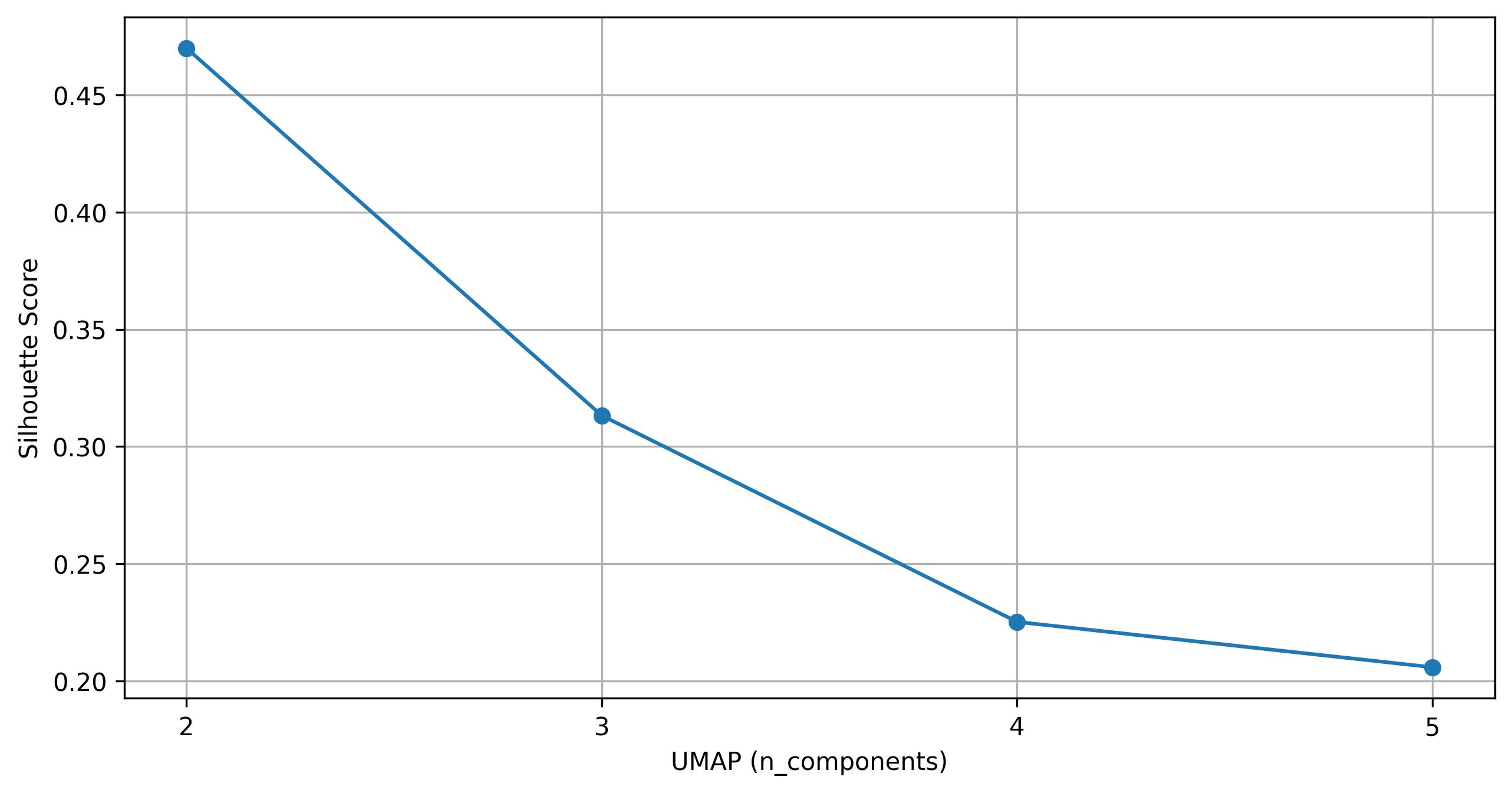
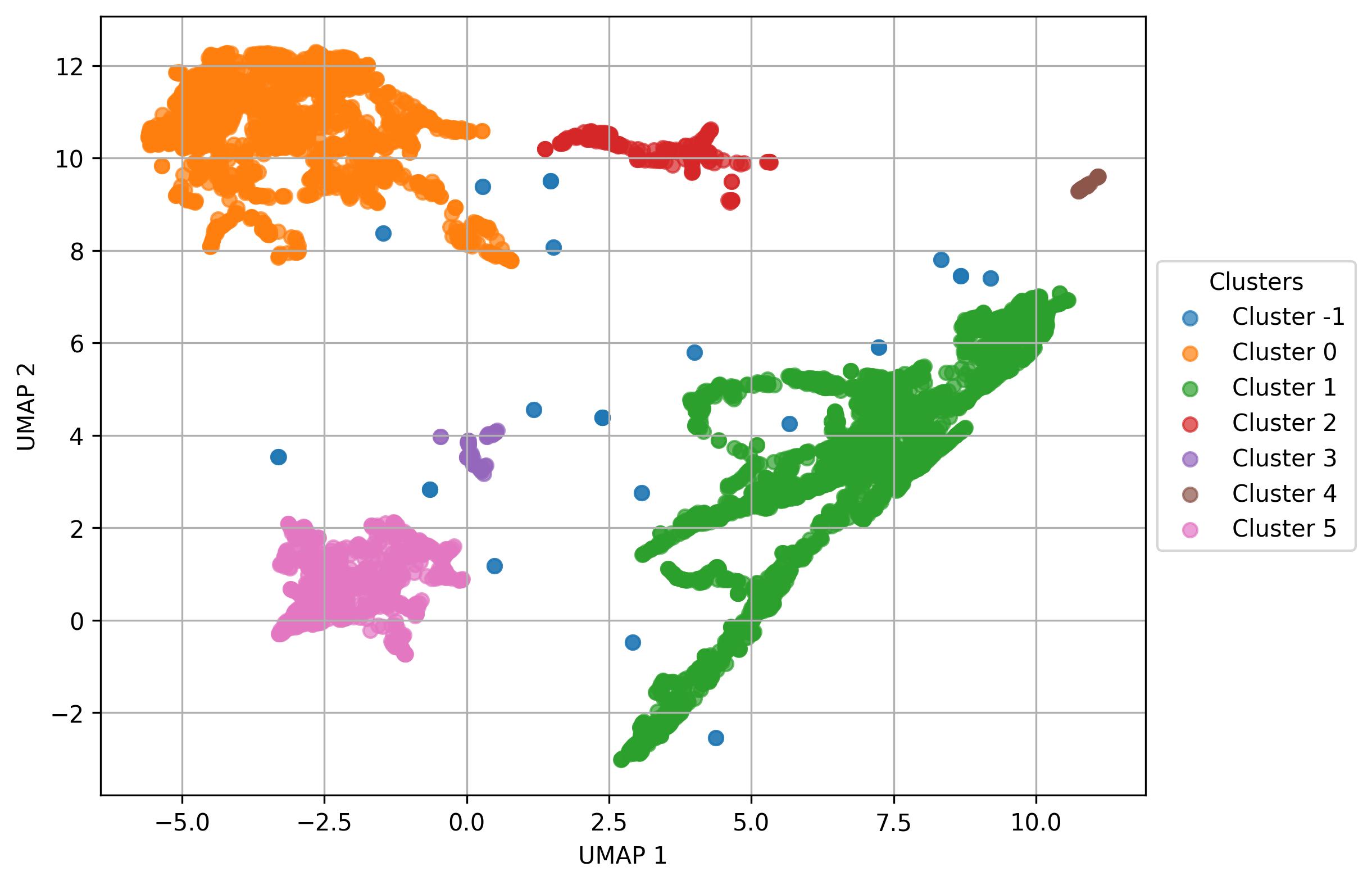
2.10. Find clusters on UMAP
fig5 = clusters.find_clusters_UMAP(
            umap_n=2,
            eps=0.5,
            min_samples=10,
            width=8,
            height=6)

clusters.return_clusters(clusters='umap')

fig5.savefig('clus_UMAP_clusters.jpeg', dpi=300, bbox_inches='tight')
2.11. Visualization of names on UMAP reduced space
fig6 = clusters.UMAP_vis(names_slot='cell_names', set_sep=True, point_size=0.6)

fig6.savefig('clus_UMAP_names_vis.jpeg', dpi=300, bbox_inches='tight')
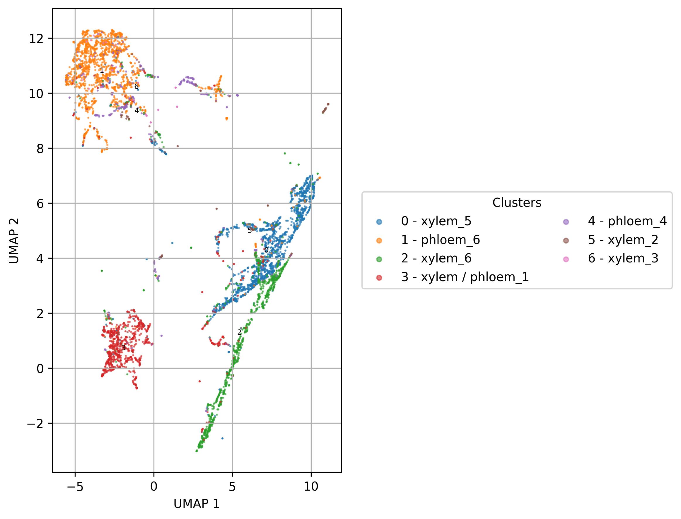
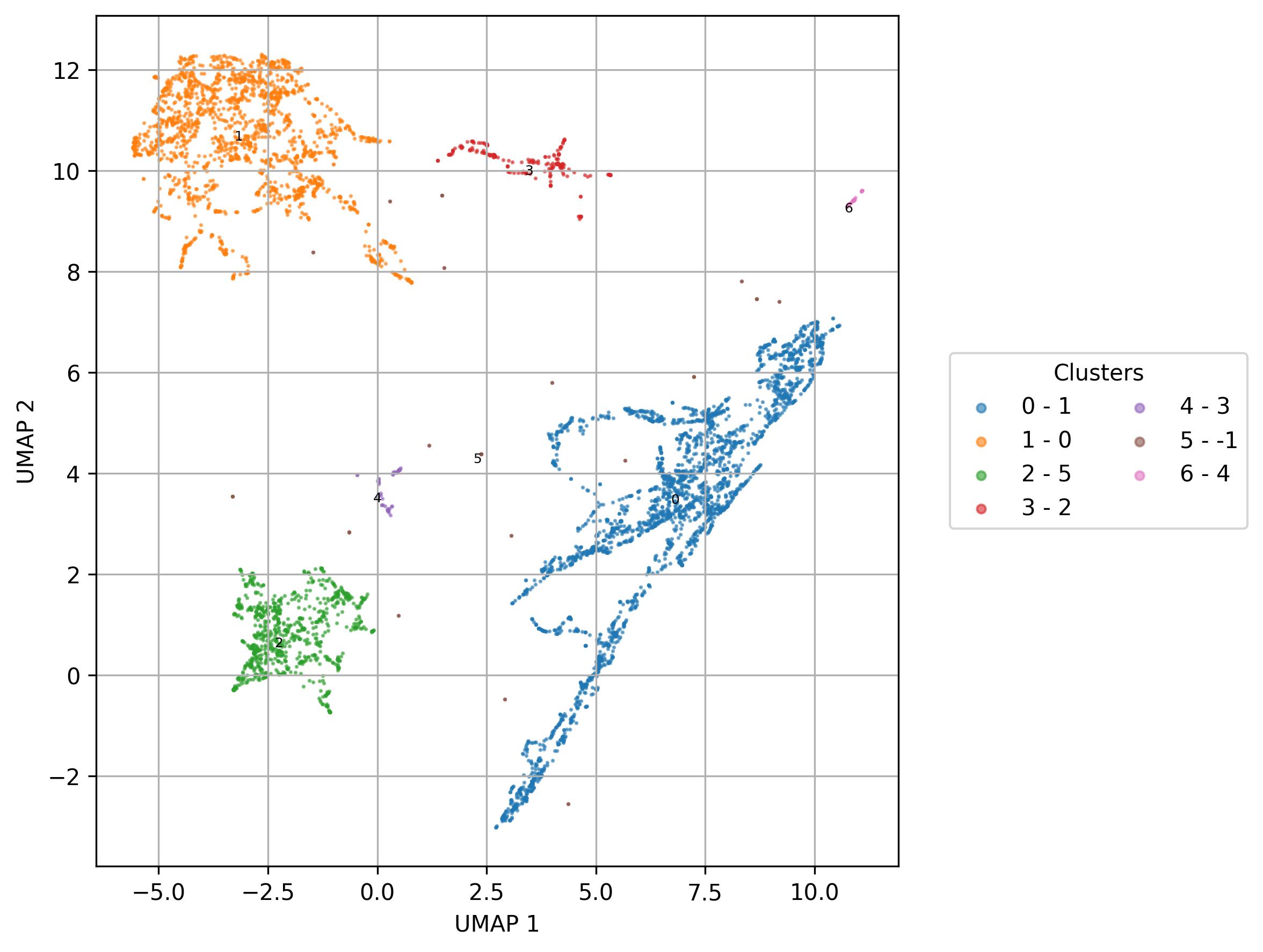
fig7 = clusters.UMAP_vis(names_slot='UMAP_clusters', set_sep=True, point_size=0.6)

fig7.savefig('clus_UMAP_clusters_vis.jpeg', dpi=300, bbox_inches='tight')
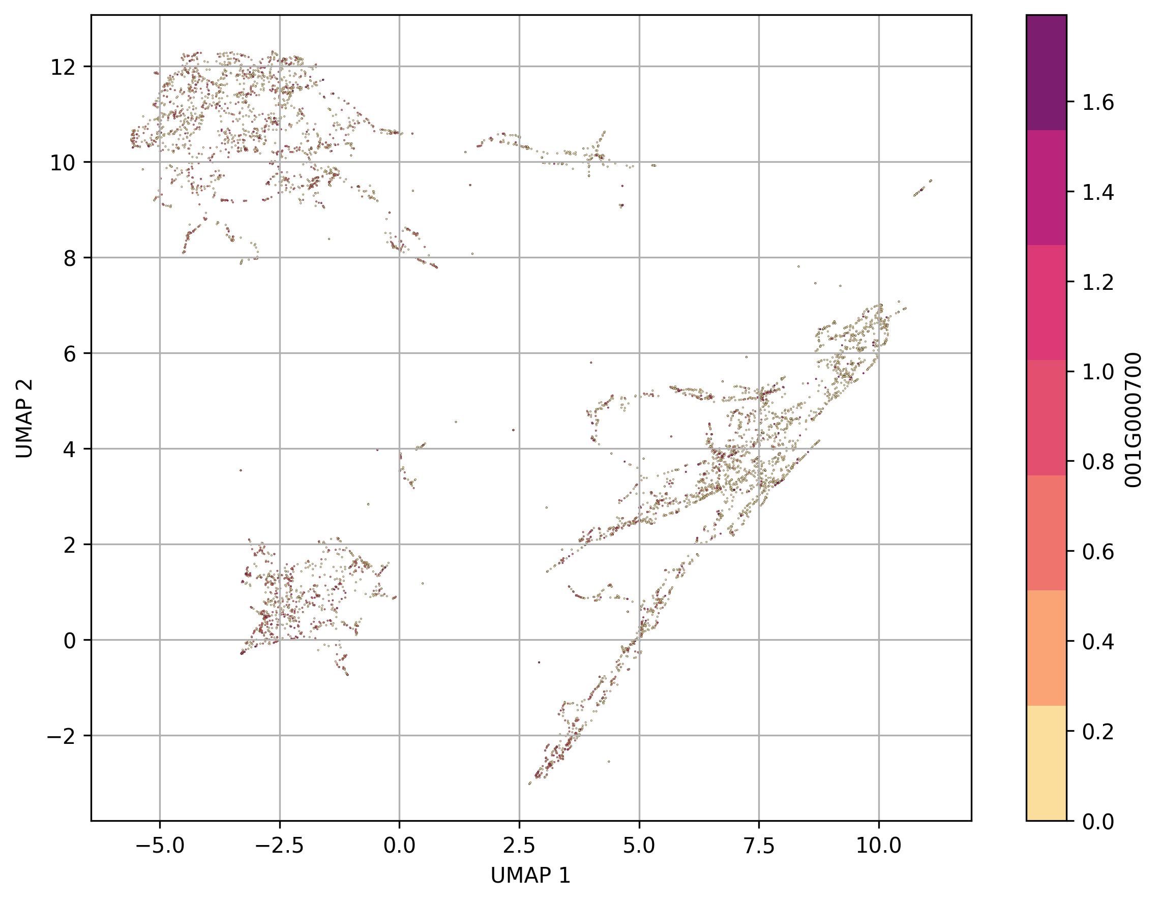
2.12. Visualization of feature level on UMAP reduced space
fig8 = clusters.UMAP_feature(
            feature_name = '001G000700',
            features_data=None,
            point_size=0.6)

fig8.savefig('clus_UMAP_features.jpeg', dpi=300, bbox_inches='tight')
3. Data integration
3.1. Loading class and helper functions
from jdti import COMPsc, volcano_plot
3.2. Initialize COMPsc class
import os

jseq_object = COMPsc.project_dir(os.getcwd(), ['set1', 'set2'])
3.3. Loading data
jseq_object.load_sparse_from_projects(normalized_data=True)

# attributes with inputed data and metadata
jseq_object.input_metadata

# if normalized_data=False
jseq_object.input_data

# if normalized_data=True
jseq_object.normalized_data
3.4. Normalize data
# use if inputed_data is count data

jseq_object.normalize_counts(normalize_factor = 100000,
                            log_transform = True)
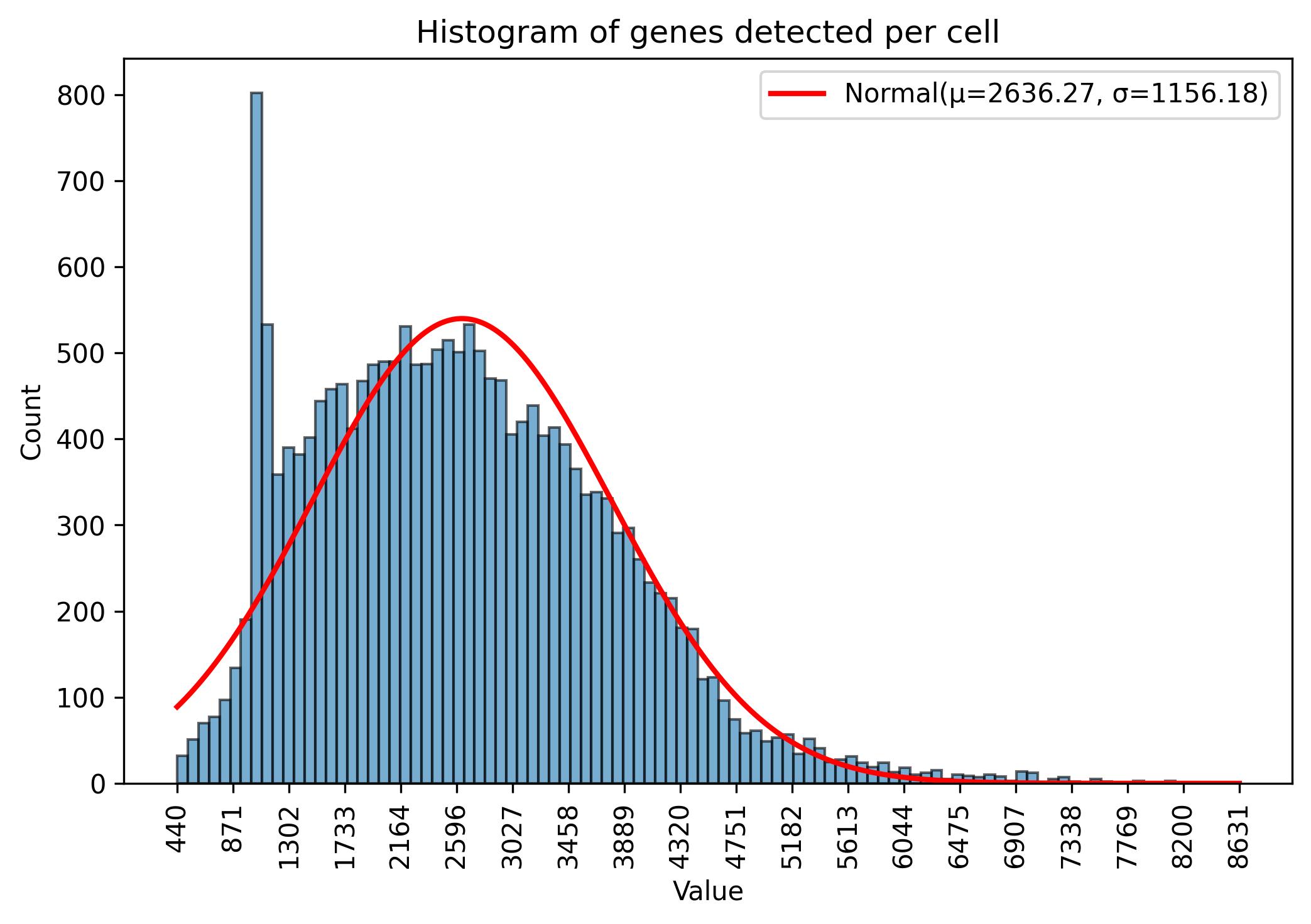
3.5. Gene amount thresholds visualisation
fig = jseq_object.gene_histograme(bins=100)

fig.savefig('int_hist_genes.jpeg', dpi=300, bbox_inches='tight')
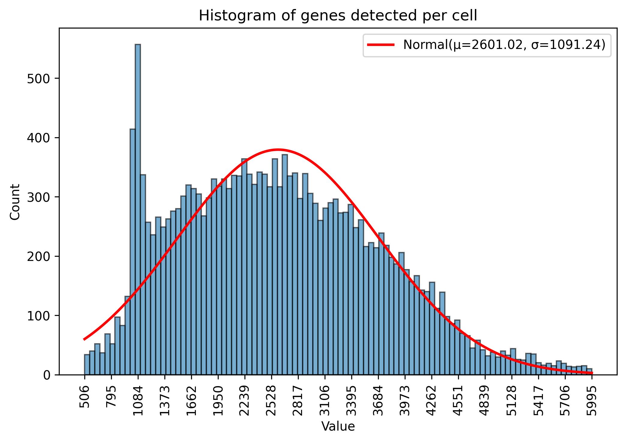
3.6. Gene amount thresholds adjustment
jseq_object.gene_threshold(min_n = 500, max_n = 6000)

fig = jseq_object.gene_histograme(bins=100)

fig.savefig('int_hist_genes_reduced.jpeg', dpi=300, bbox_inches='tight')
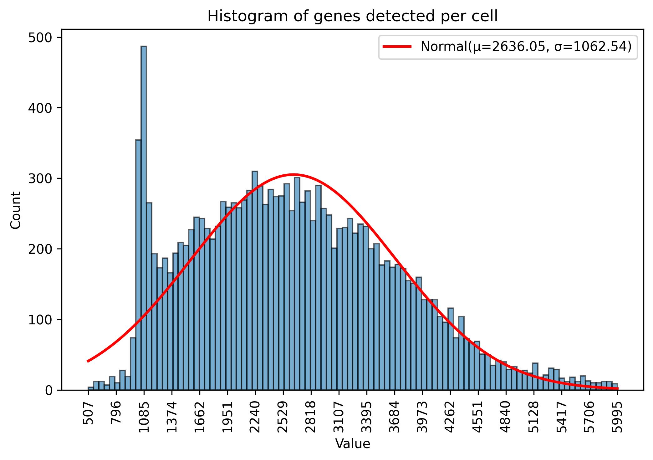
3.7. Sample reduction
jseq_object.reduce_cols(reg = 'xylem / phloem', inc_set = False)

fig = jseq_object.gene_histograme(bins=100)

fig.savefig('int_hist_genes_reduced_names.jpeg', dpi=300, bbox_inches='tight')
3.8. Samples / cells amount visualisation
fig = jseq_object.cell_histograme(name_slot = 'cell_names')

fig.savefig('int_hist_cell_names.jpeg', dpi=300, bbox_inches='tight')
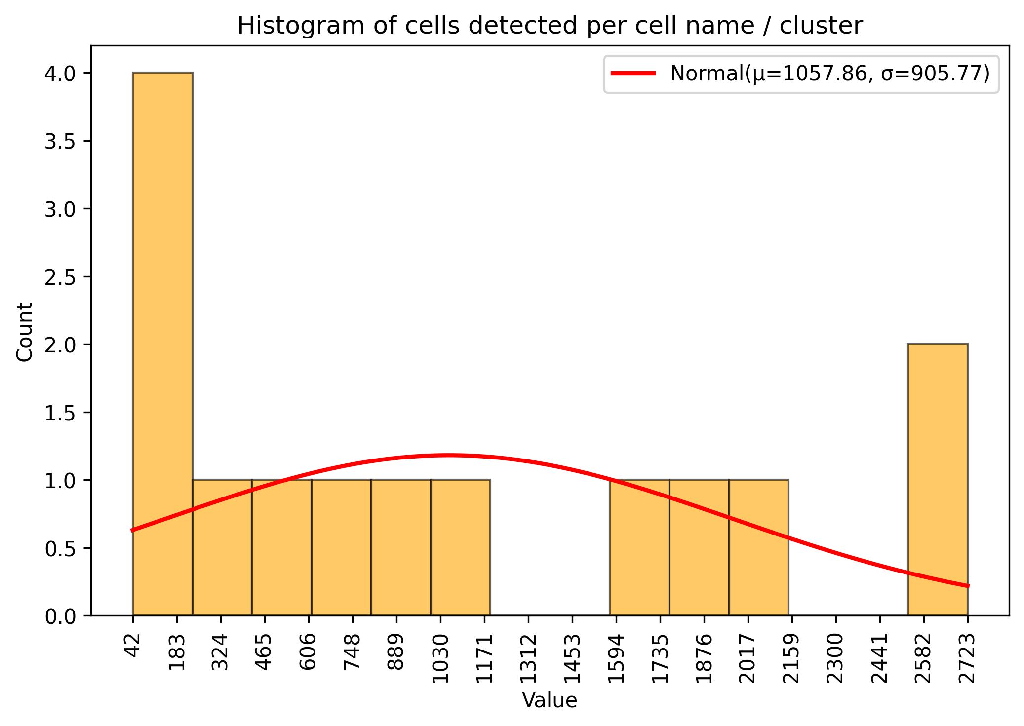
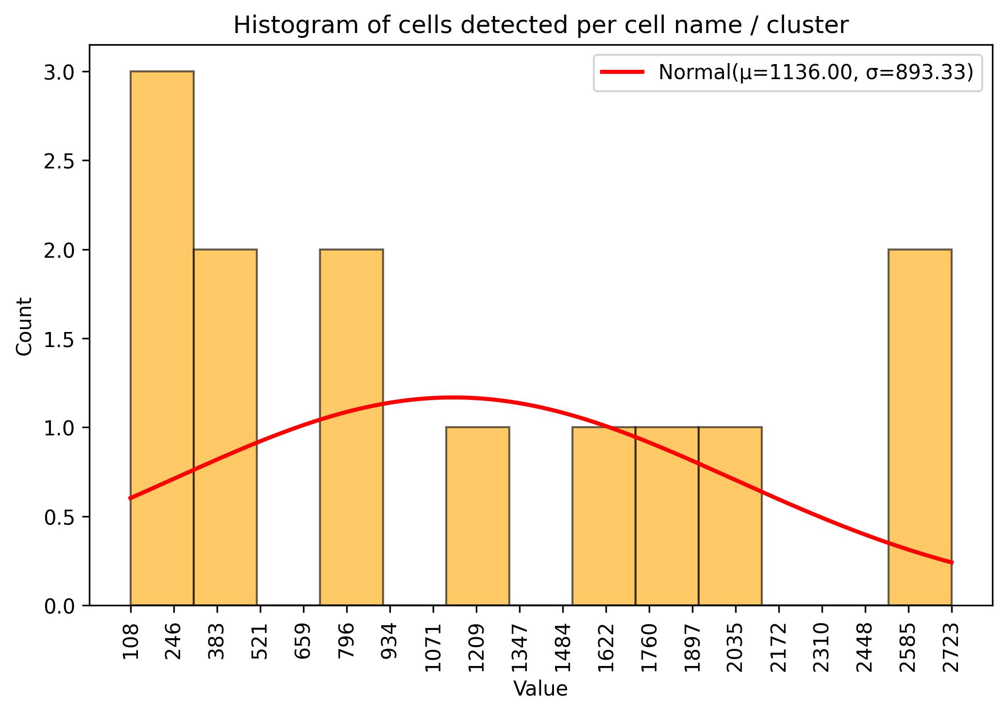
3.9. Sample / cell amount threshold
jseq_object.cluster_threshold(min_n = 50, name_slot = 'cell_names')

fig = jseq_object.cell_histograme(name_slot = 'cell_names')

fig.savefig('int_hist_cell_names_reduced.jpeg', dpi=300, bbox_inches='tight')
3.10. Calculation of differential markers for integration
jseq_object.calculate_difference_markers(min_exp = 0,
                                         min_pct = 0.25,
                                         n_proc=10,
                                         force = False)
3.11. Calculation of samples / cells similarity factors
jseq_object.estimating_similarity(method = 'pearson',
                                  p_val = 0.05,
                                  top_n = 25)
3.12. Similarity visualisation (correlation x distance)
fig1 = jseq_object.similarity_plot(split_sets = True,
                                 set_info = True,
                                 cmap='seismic',
                                 width = 8, height = 5)

fig1.savefig('int_sim_plot_top.jpeg', dpi=300, bbox_inches='tight')
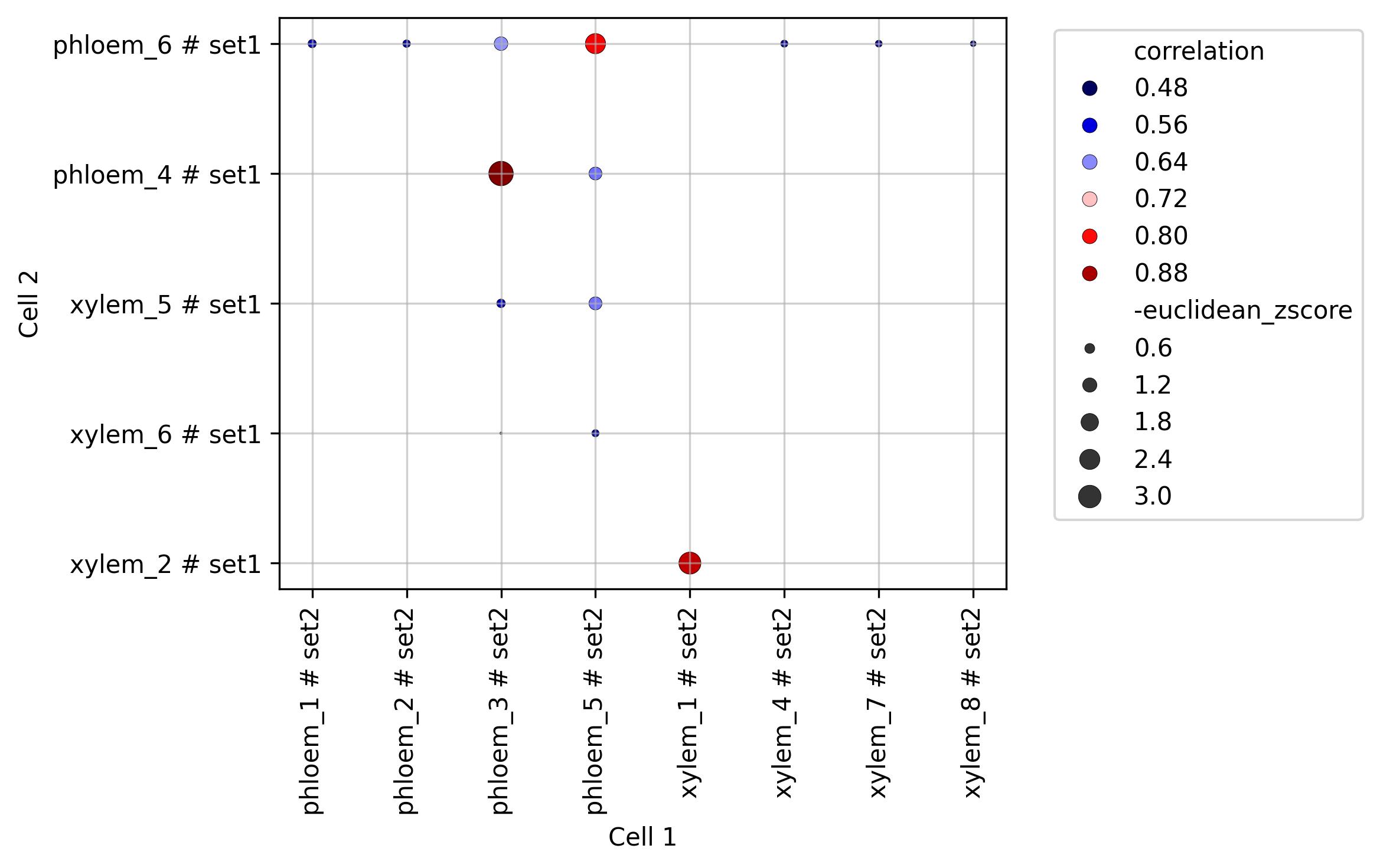
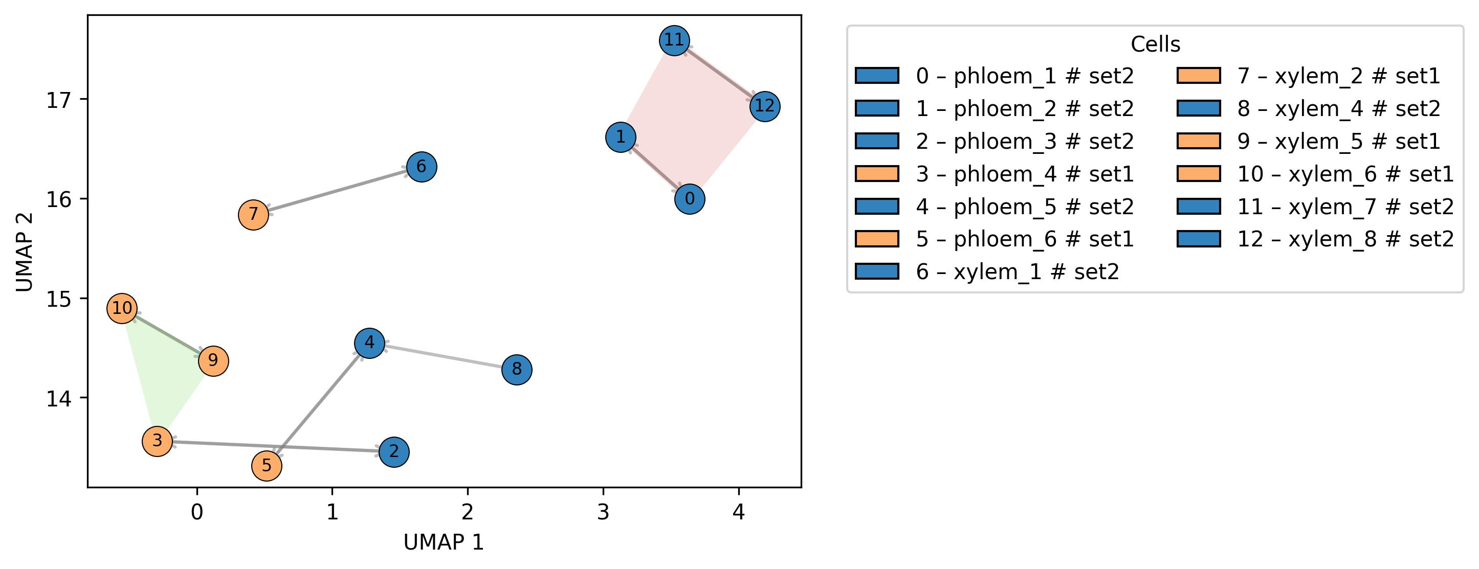
3.13. Similarity visualisation (spatial distance)
fig2 = jseq_object.spatial_similarity(set_info= True,
                                     bandwidth = 1,
                                        n_neighbors = 6,
                                        min_dist = 0.5,
                                        legend_split = 2,
                                        point_size = 200,
                                        spread=1.0,
                                        set_op_mix_ratio=1.0,
                                        local_connectivity=1,
                                        repulsion_strength=1.0,
                                        negative_sample_rate=5,
                                        width = 6,
                                        height = 4)


fig2.savefig('int_sim_plot_map_top.jpeg', dpi=300, bbox_inches='tight')
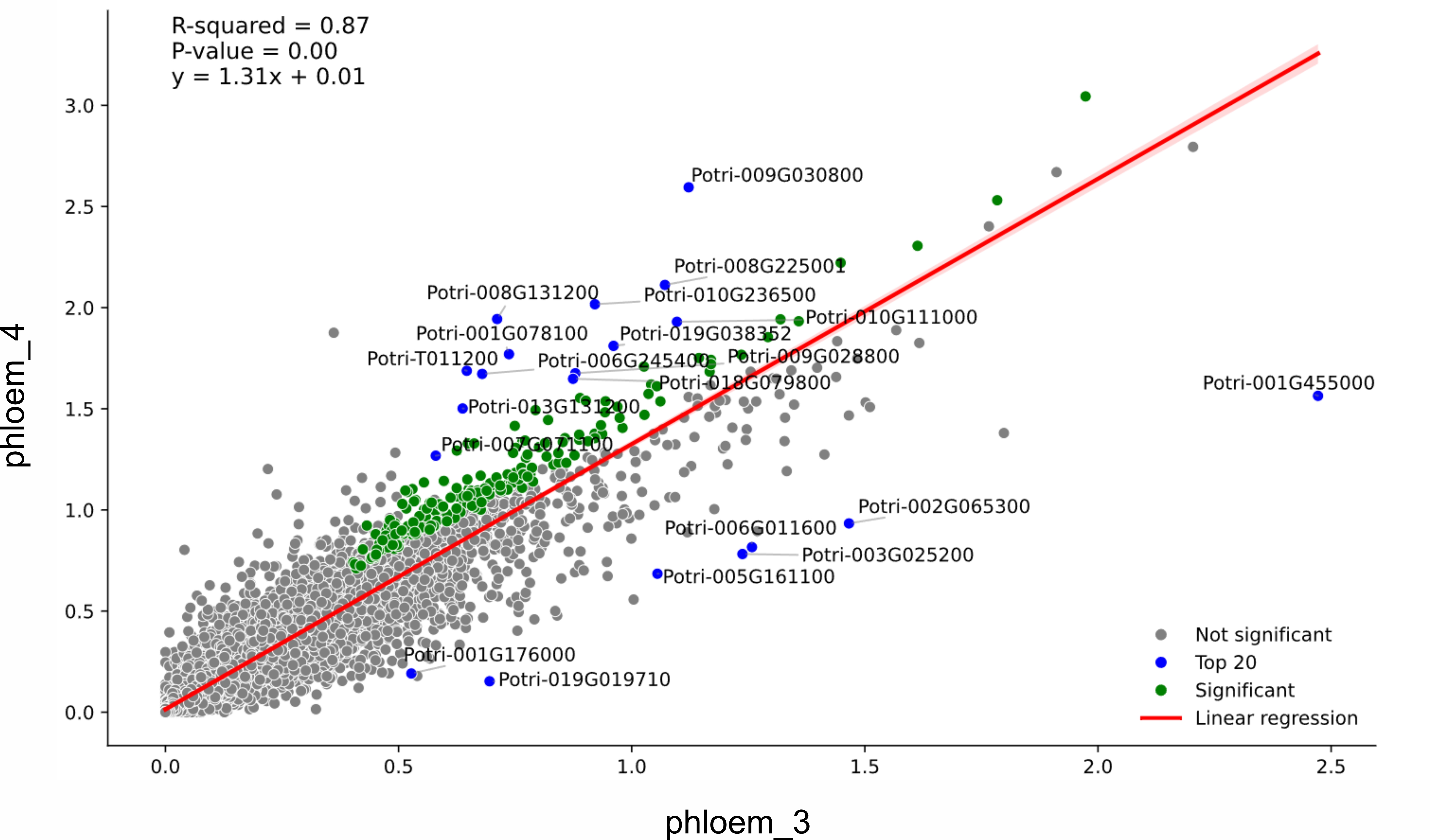
3.14. Similarity visualisation (sample to sample)
df, fig3 = jseq_object.cell_regression(
        cell_x="phloem_4",
        cell_y="phloem_3",
        set_x="set1",
        set_y="set2",
        min_log=0.5,
        n_max=20,
        min_exp=0.1,
        min_pct=0.5,
        n_proc=10,
        min_esm=0.5,
        p_val=0.05,
        adj=True,
        image_width=12,
        image_high=7,
    )

fig3.savefig('int_sim_reg.jpeg', dpi=300, bbox_inches='tight')
3.15. Analysis of cluster dispersion
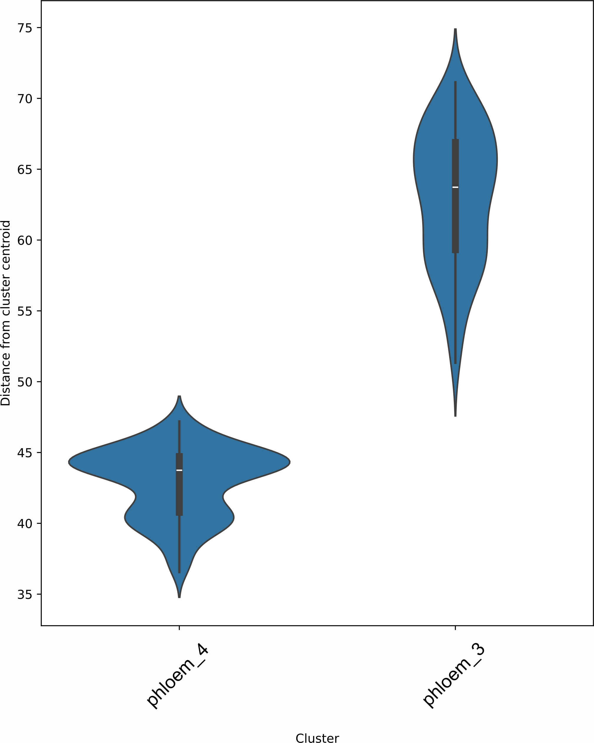
3.15.1 Distance from centroide - violin plot
fig3_1 = jseq_object.cell_dispersion(
        cells_names=["phloem_4", "phloem_3"],
        cells_sets=None,
        image_width=7,
        image_high=10
    )


fig3_1.savefig('dispersion.jpeg', dpi=300, bbox_inches='tight')
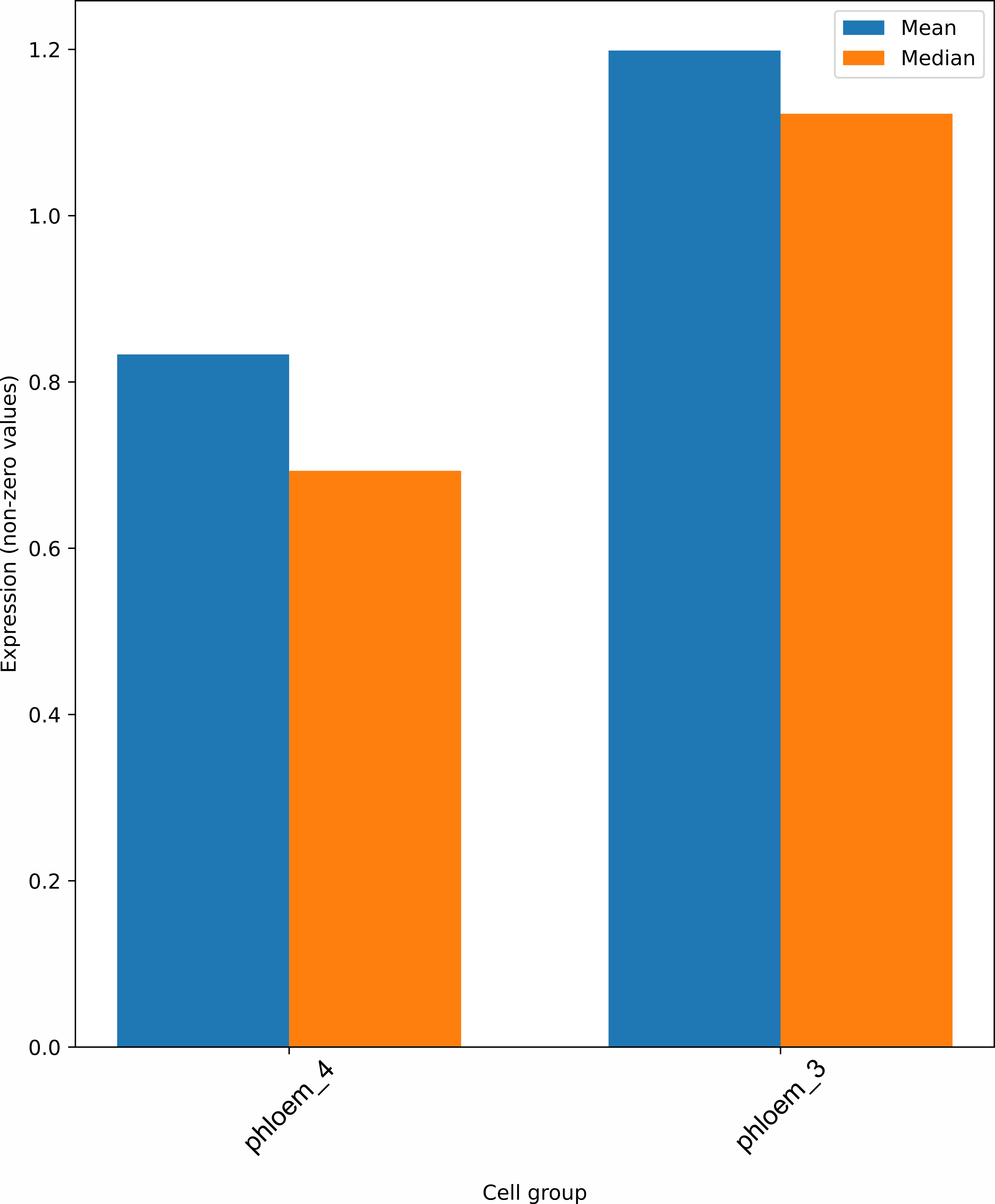
3.15.2 Mean / median number of genes per cluster - bar plot
fig3_2 = jseq_object.mm_cell_genes(
        cells_names=["phloem_4", "phloem_3"],
        cells_sets=None,
        non_include_zeros=True,
        image_width=7,
        image_high=10,
    )

fig3_2.savefig('mean_median_genes.jpeg', dpi=300, bbox_inches='tight')
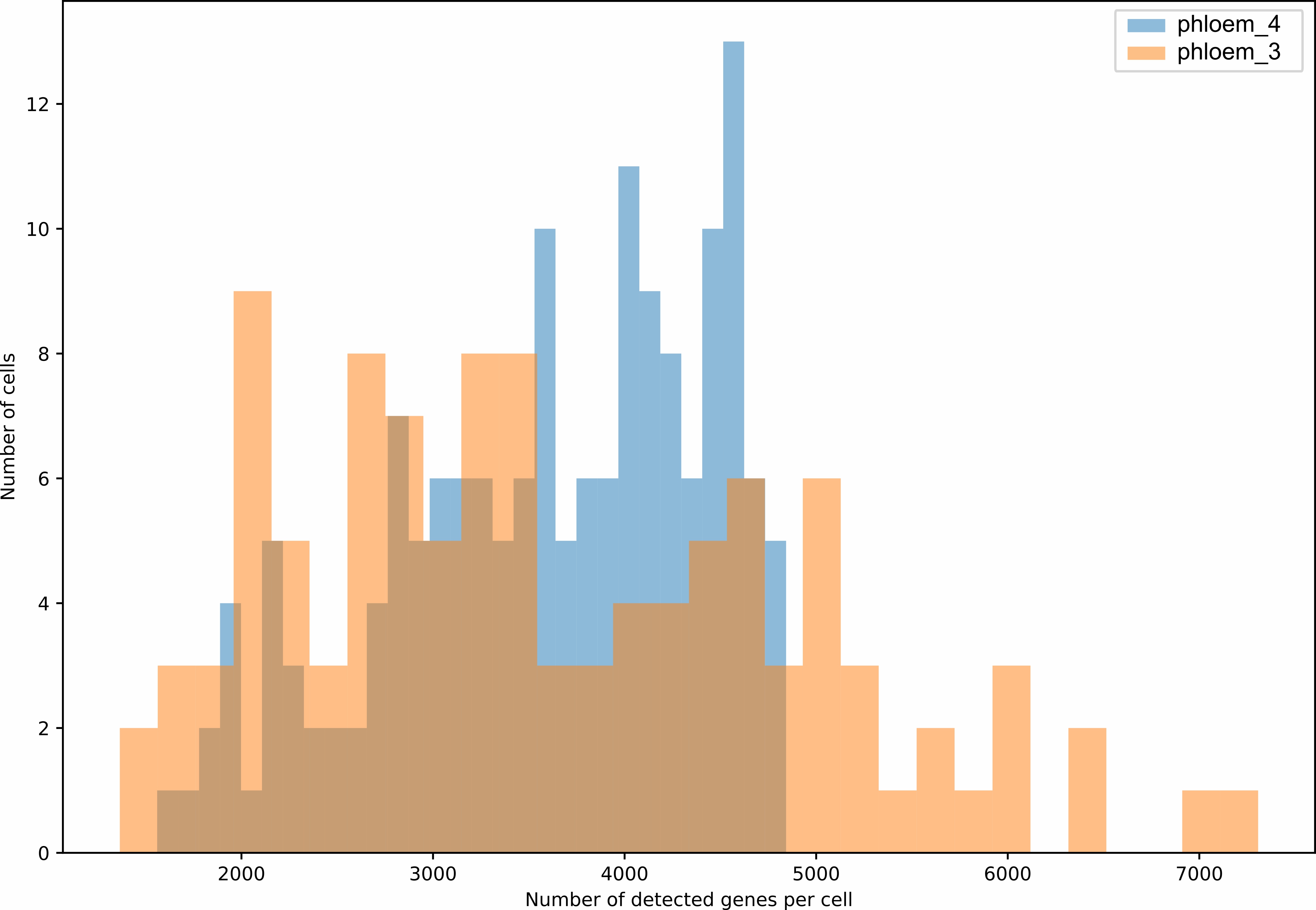
3.15.3 Genes distribution in selected clusters - histograme
fig3_3 = jseq_object.cell_genes_distribution(
        cells_names=["phloem_4", "phloem_3"],
        cells_sets=None,
        image_width=10,
        image_high=7
    )

fig3_3.savefig('genes_distribution.jpeg', dpi=300, bbox_inches='tight')
3.16. Clustering features estimation
jseq_object.clustering_features(name_slot = 'cell_names',
                                features_list = None,
                                p_val = 0.05,
                                top_n = 25,
                                adj_mean = True,
                                beta = 0.2)
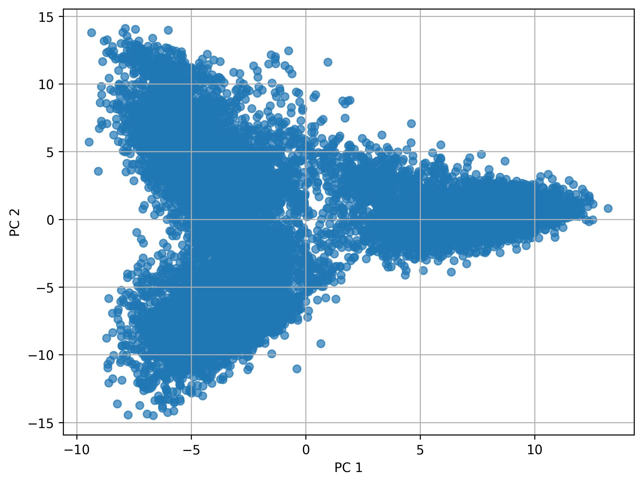
3.17. Performing PCA
fig4 = jseq_object.perform_PCA(pc_num = 50)

fig4.savefig('int_pca.jpeg', dpi=300, bbox_inches='tight')
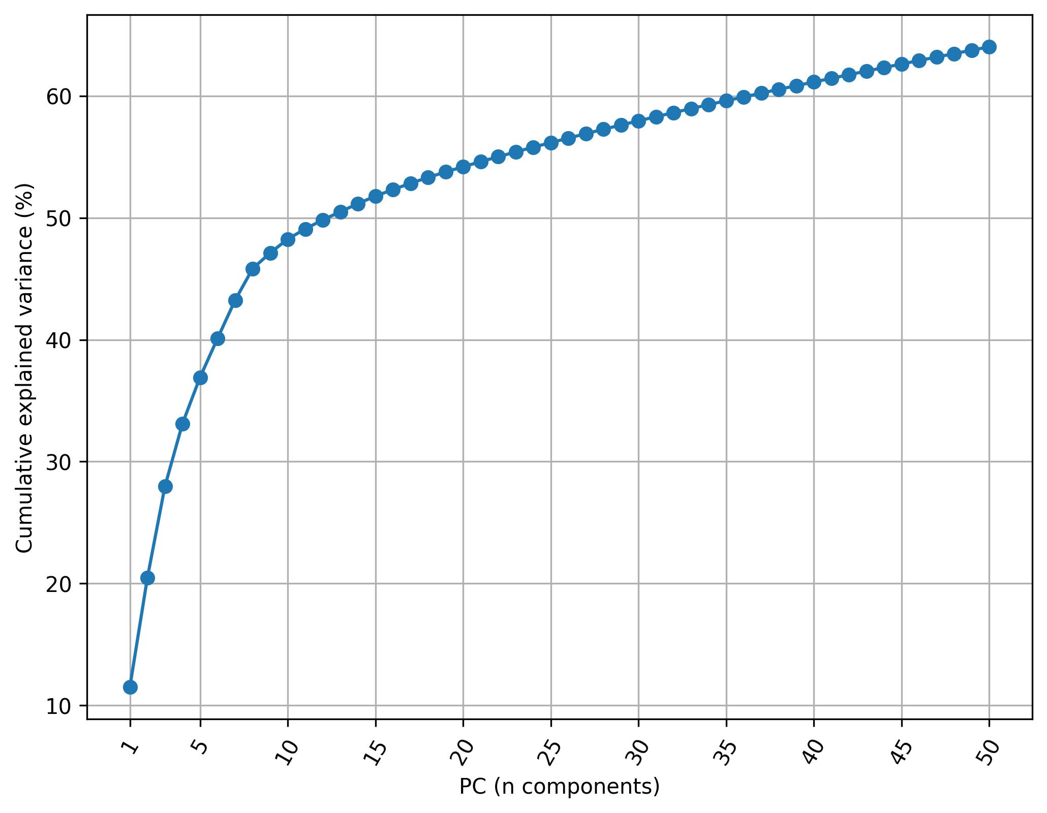
3.18. Knee plot of PC
fig5 = jseq_object.knee_plot_PCA()

fig5.savefig('int_pca_knee.jpeg', dpi=300, bbox_inches='tight')
3.19. Harmonize data (Harmony)
# if more than one dataset (provided in metadata) harmonization
# process for integration element can be used

jseq_object.harmonize_sets()
3.20. Perform UMAP
jseq_object.perform_UMAP(factorize=False,
                        umap_num = 2,
                        pc_num = 15,
                        harmonized = True)
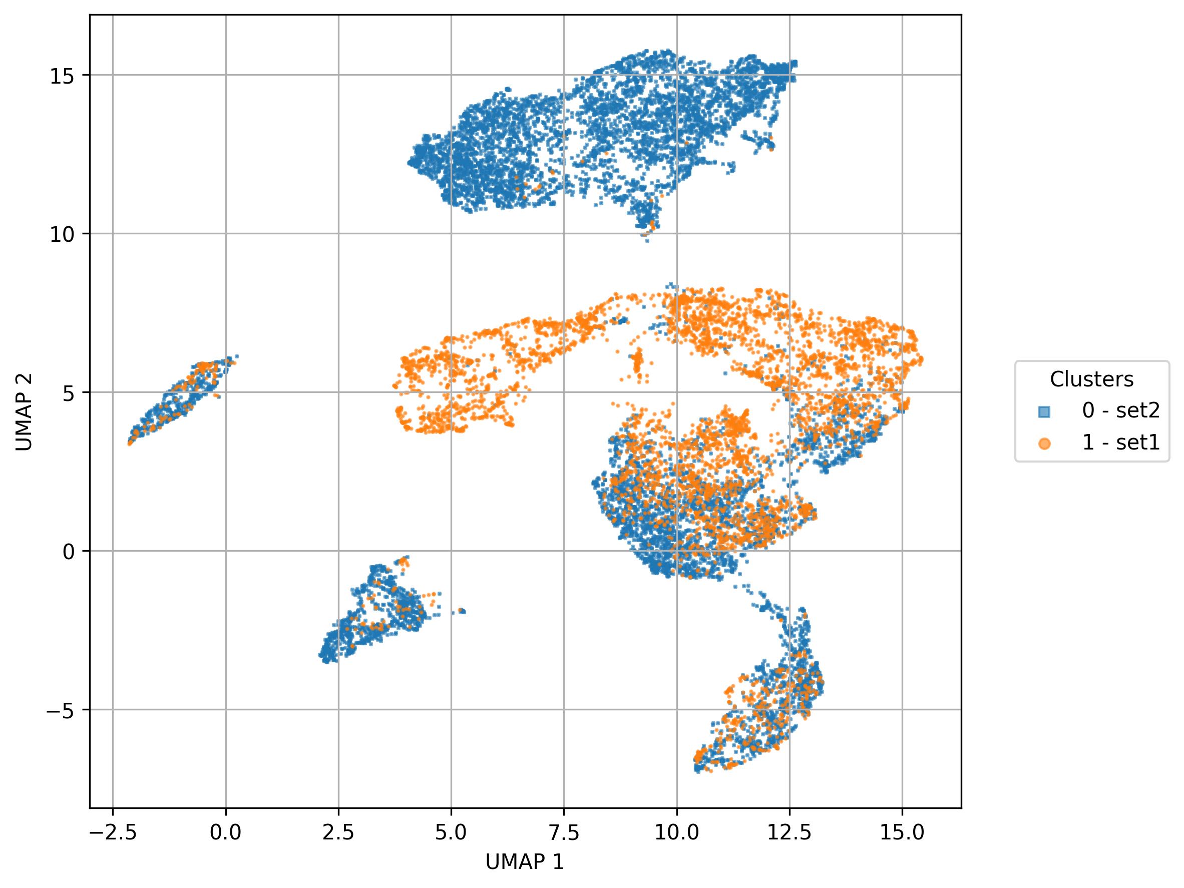
3.21. Visualization of names / sets on UMAP reduced space
fig6 = jseq_object.UMAP_vis(
             names_slot = 'cell_names',
             set_sep = True,
             point_size = 1,
             font_size = 10,
             legend_split_col = 1,
             width = 8,
             height = 6,
             inc_num = True)


fig6.savefig('int_umap.jpeg', dpi=300, bbox_inches='tight')
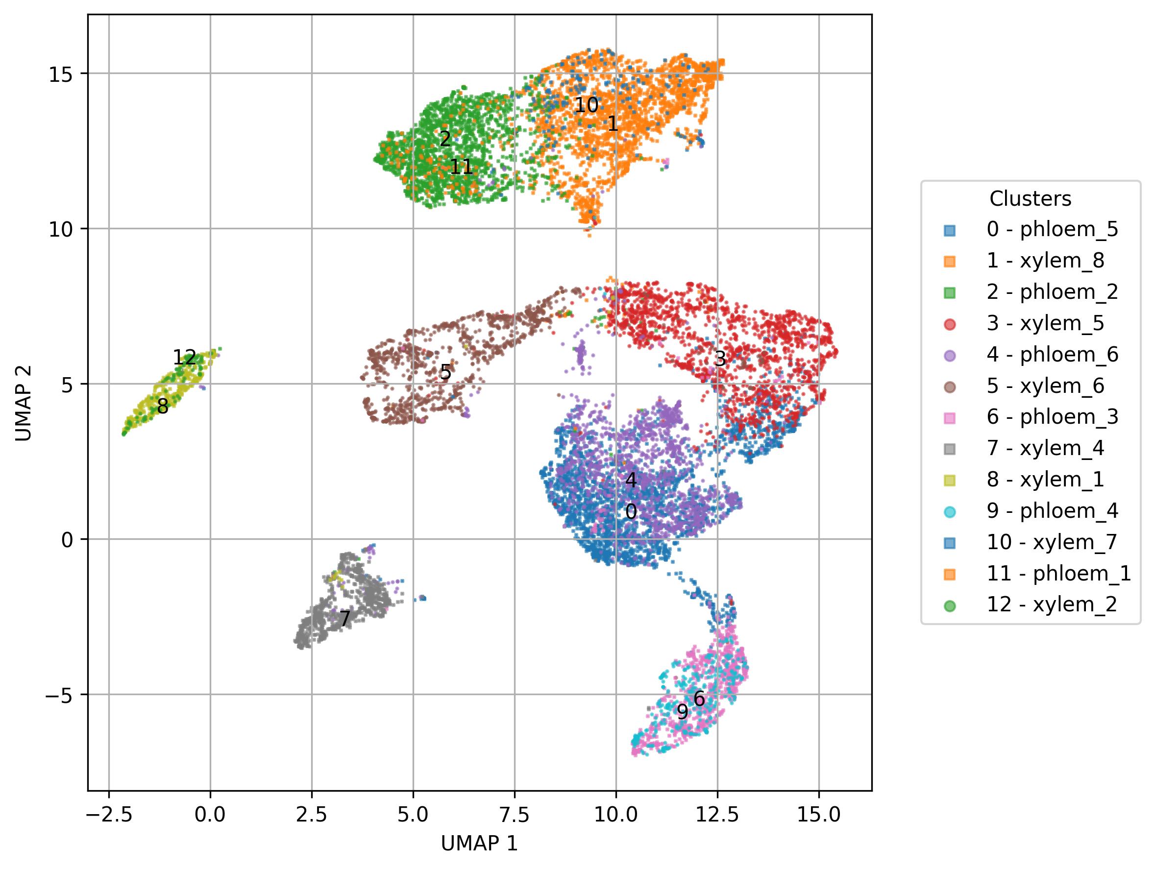
fig7 = jseq_object.UMAP_vis(
             names_slot = 'sets',
             set_sep = True,
             point_size = 1,
             font_size = 6,
             legend_split_col = 1,
             width = 8,
             height = 6,
             inc_num = False)

fig7.savefig('int_umap_sets.jpeg', dpi=300, bbox_inches='tight')
3.22. Visualization of feature level on UMAP reduced space
fig8 = jseq_object.UMAP_feature(
             features_data = jseq_object.get_data(set_info = False) ,
             feature_name = '001G069799',
             point_size = 0.8,
             font_size = 6,
             width = 8,
             height = 6,
             palette = 'light')

fig8.savefig('int_umap_feature.jpeg', dpi=300, bbox_inches='tight')
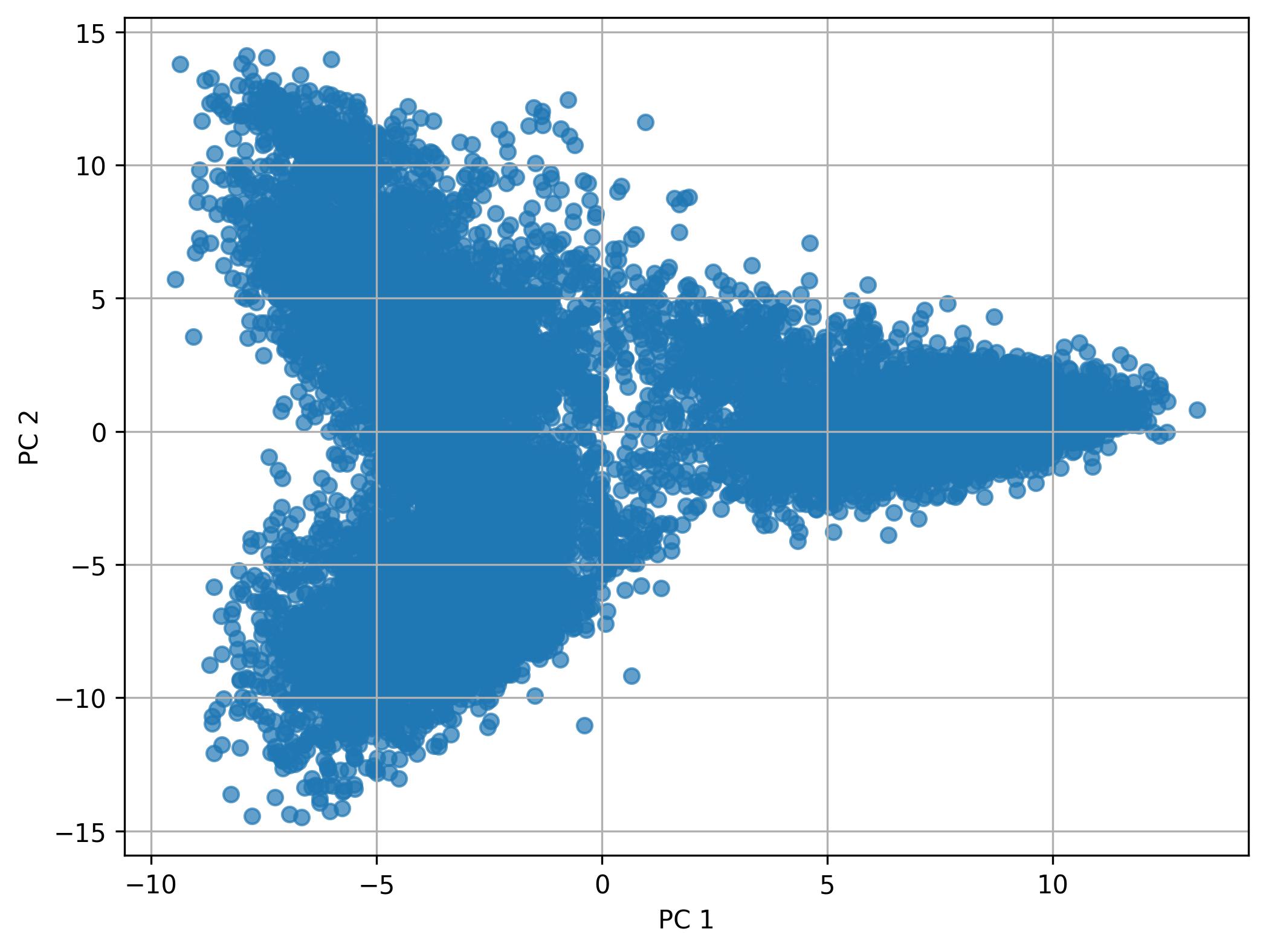
3.23. De novo clustering - Performing PCA
fig9 = jseq_object.perform_PCA(pc_num = 50)

fig9.savefig('int_pca_clusters.jpeg', dpi=300, bbox_inches='tight')
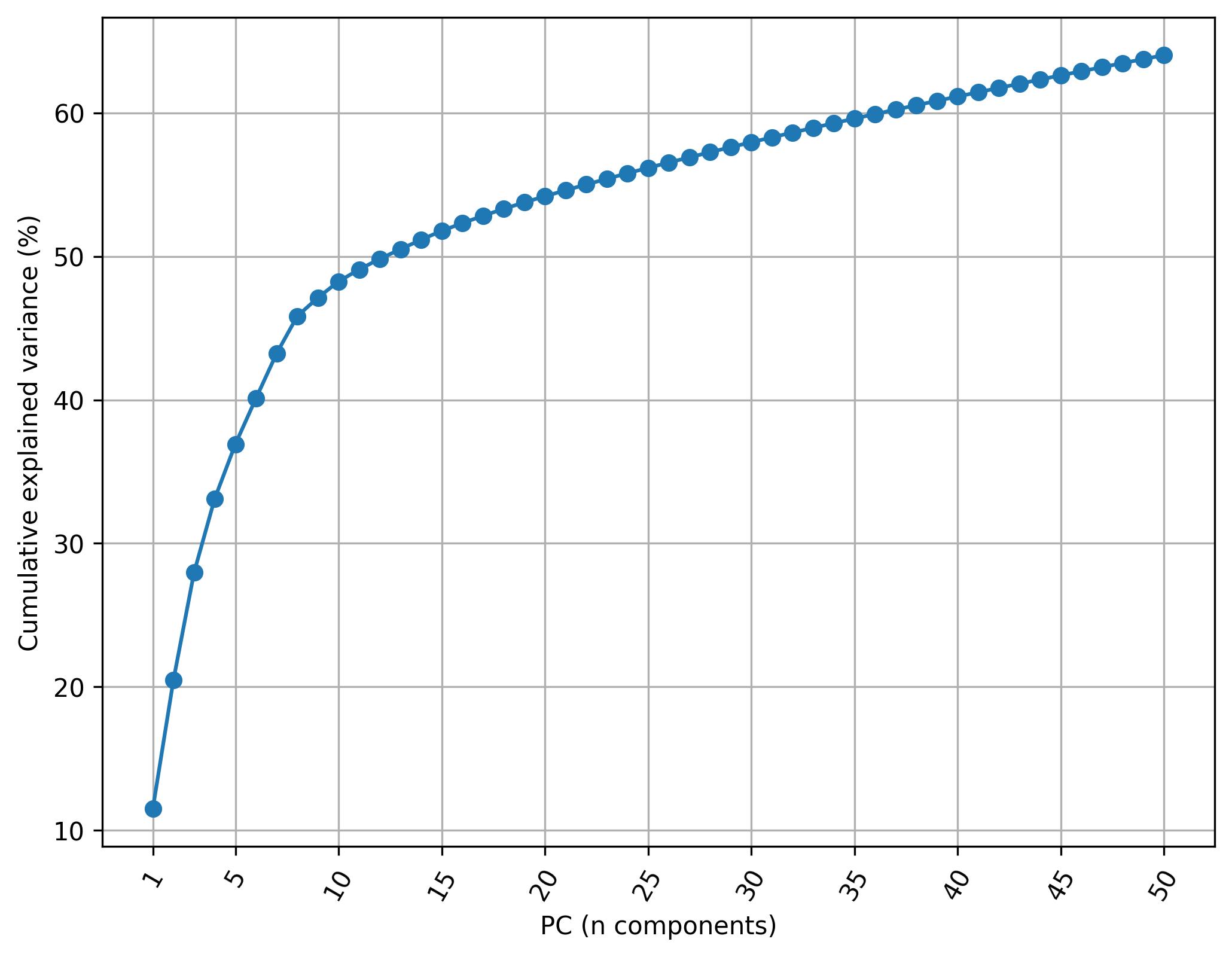
3.24. De novo clustering - Knee plot of PC
fig10 = jseq_object.knee_plot_PCA()

fig10.savefig('int_pca_knee_clusters.jpeg', dpi=300, bbox_inches='tight')
3.25. De novo clustering - Harmonize data (Harmony)
# if more than one dataset (provided in metadata) harmonization
# process for integration element can be used

jseq_object.harmonize_sets()
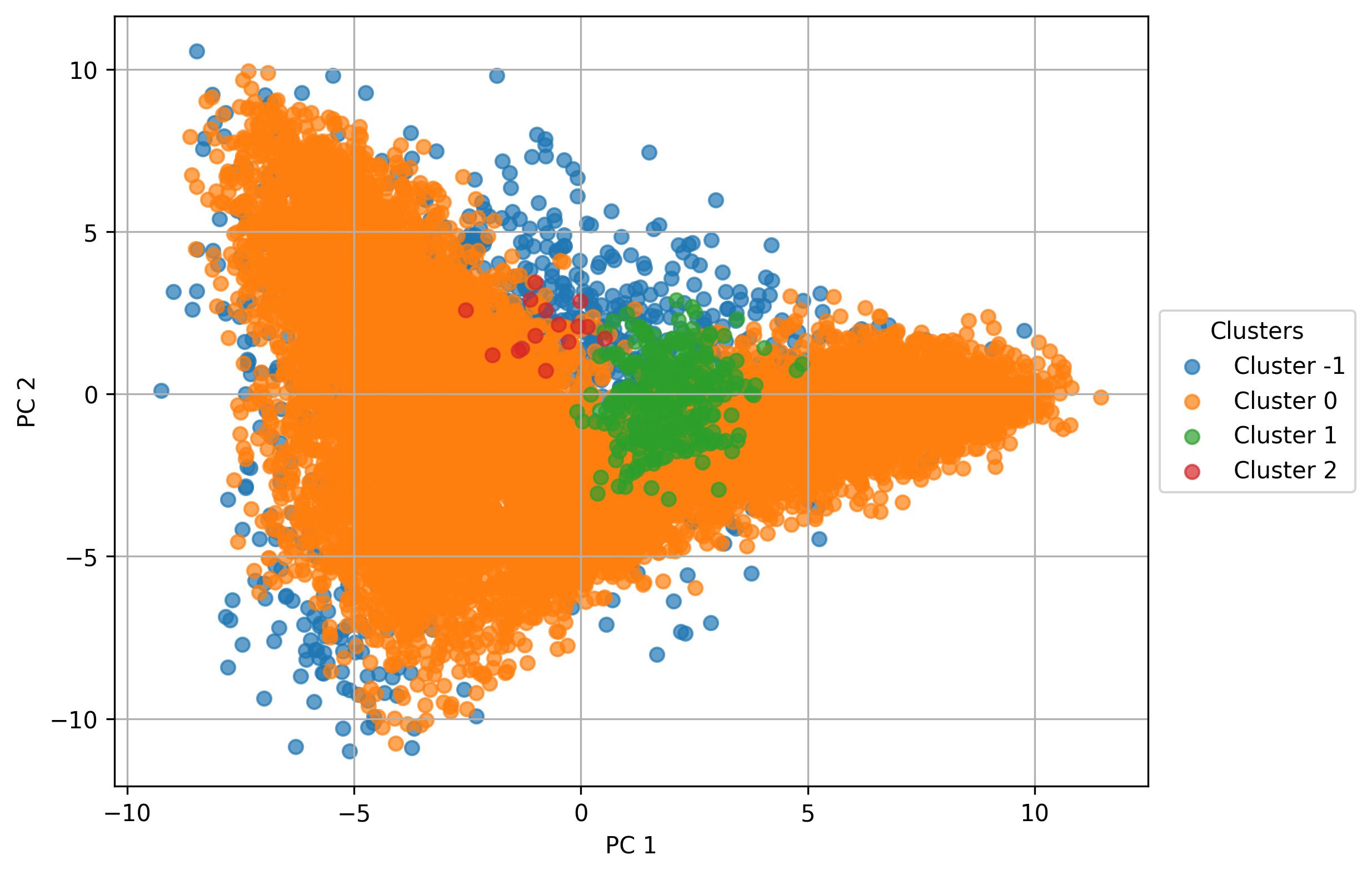
3.26. De novo clustering - Find clusters on PC
fig11 = jseq_object.find_clusters_PCA(
                        pc_num = 10,
                        eps = 3,
                        min_samples = 20,
                        harmonized = True)

fig11.savefig('int_pca_clusters_find.jpeg', dpi=300, bbox_inches='tight')
3.27. De novo clustering - Perform UMAP
jseq_object.perform_UMAP(
                factorize=False,
                umap_num = 10,
                pc_num = 10,
                harmonized = True)
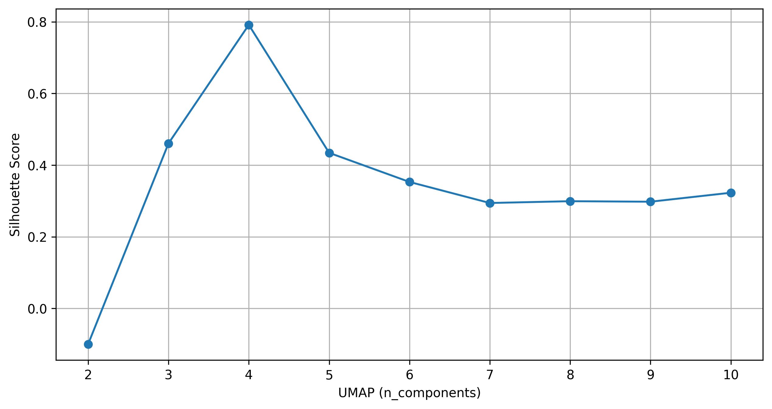
3.28. De novo clustering - Knee plot of UMAP
fig12 = jseq_object.knee_plot_umap(eps = 0.5, min_samples = 10)

fig12.savefig('int_umap_knee.jpeg', dpi=300, bbox_inches='tight')
3.29. De novo clustering - Find clusters on UMAP
fig13 = jseq_object.find_clusters_UMAP(umap_n = 4,
                              eps = 0.5,
                              min_samples = 10,
                              width = 8,
                              height = 6)

fig13.savefig('int_umap_clusters.jpeg', dpi=300, bbox_inches='tight')
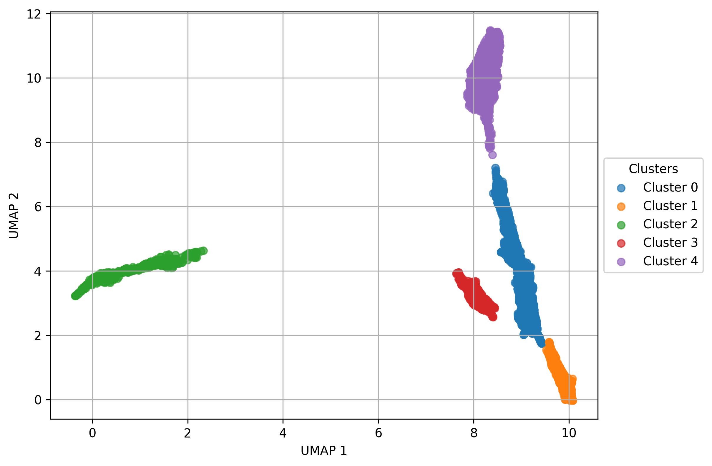
3.30. De novo clustering - Visualization of clusters on UMAP reduced space
fig14 = jseq_object.UMAP_vis(
             names_slot = 'UMAP_clusters',
             set_sep = True,
             point_size = 1,
             font_size = 10,
             legend_split_col = 1,
             width = 8,
             height = 6,
             inc_num = True)

fig14.savefig('int_umap_clusters_get_clusters_sep_set.jpeg', dpi=300, bbox_inches='tight')
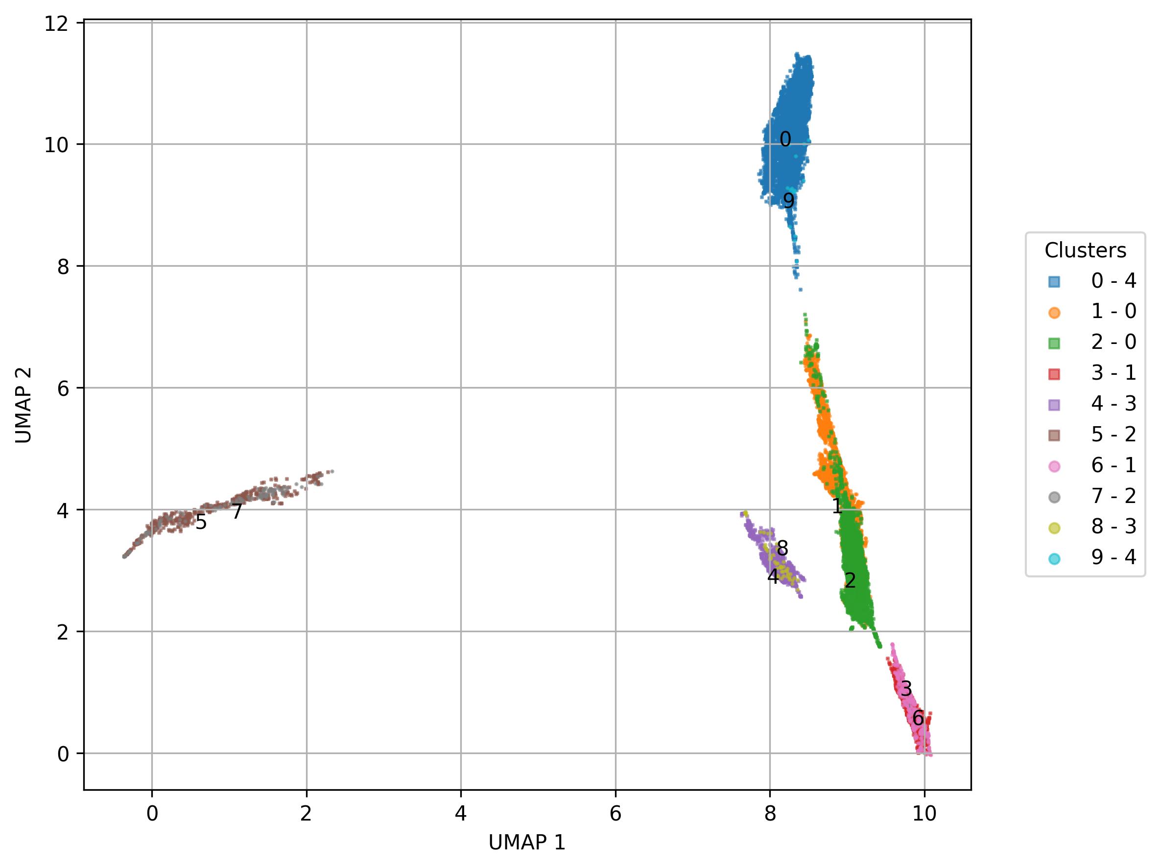
fig15 = jseq_object.UMAP_vis(
             names_slot = 'UMAP_clusters',
             set_sep = False,
             point_size = 1,
             font_size = 10,
             legend_split_col = 1,
             width = 8,
             height = 6,
             inc_num = True)


fig15.savefig('int_umap_clusters_get_clusters_sep_set_not.jpeg', dpi=300, bbox_inches='tight')
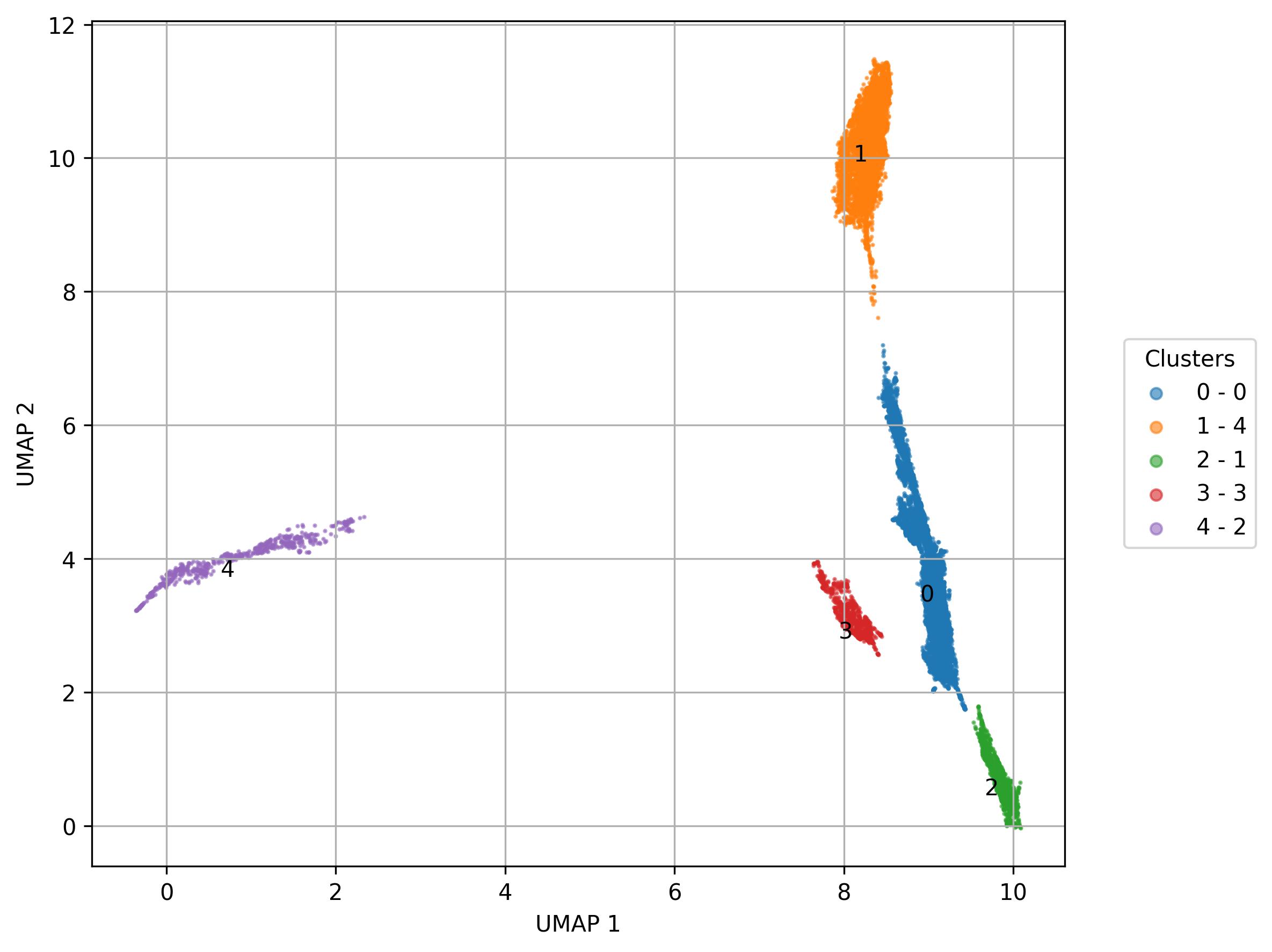
3.31. Differential expression analysis
# if you want calculate markers for de novo clusters change metadata 'cell_names'
# jseq_object.input_metadata['cell_names'] = jseq_object.input_metadata['UMAP_clusters']

# calculation stats for all cells in 'cell_anmes'
stats = jseq_object.statistic(cells='All', sets=None, min_exp=0, min_pct=0.25, n_proc=10)

# calculation stats for all clusters in 'UMAP_clusters'
cell_names = jseq_object.input_metadata['cell_names'] # save cell_names for the future
jseq_object.input_metadata['cell_names'] = jseq_object.input_metadata['UMAP_clusters']
stats = jseq_object.statistic(cells='All', sets=None, min_exp=0, min_pct=0.25, n_proc=10)
# calculation stats for all sets in 'sets',

stats = jseq_object.statistic(cells=None, sets='All', min_exp=0, min_pct=0.25, n_proc=10)
- DEG data:
feature– Name of the studied featurep_val– P-value (Mann–Whitney) for the studied feature comparing thevalid_groupto all other groups in the analysispct_valid– Percentage of positive (>0) values for the studied feature in thevalid_group*pct_ctrl– Percentage of positive (>0) values for the studied feature in all other groupsavg_valid– Average value of the studied feature in thevalid_groupavg_ctrl– Average value of the studied feature in the remaining groupssd_valid– Standard deviation of the studied feature in thevalid_group*sd_ctrl– Standard deviation of the studied feature in the remaining groupsesm– Cohen’s d effect size metricvalid_group– Name of the sample or group belonging to thevalid_groupadj_pval– Benjamini–Hochberg adjusted p-valueFC– Fold change between the averagedvalid_groupsamples and the averaged remaining sampleslog(FC)– Log₂-transformed fold changenorm_diff– Direct difference between the averagedvalid_groupvalue and the averaged value of the remaining groups
3.32. Volcano plot
# select 'valid_group' for volcano plot create; this case 'set1' or 'set2'
stats_volcano = stats[stats['valid_group'] == 'set1']

fig16 = volcano_plot(deg_data = stats_volcano,
                  p_adj = True,
                  top = 10,
                  p_val = 0.05,
                  lfc = 0.25,
                  standard_scale = False,
                  rescale_adj = True,
                  image_width = 12,
                  image_high = 13)

fig16.savefig('int_volcano.jpeg', dpi=300, bbox_inches='tight')
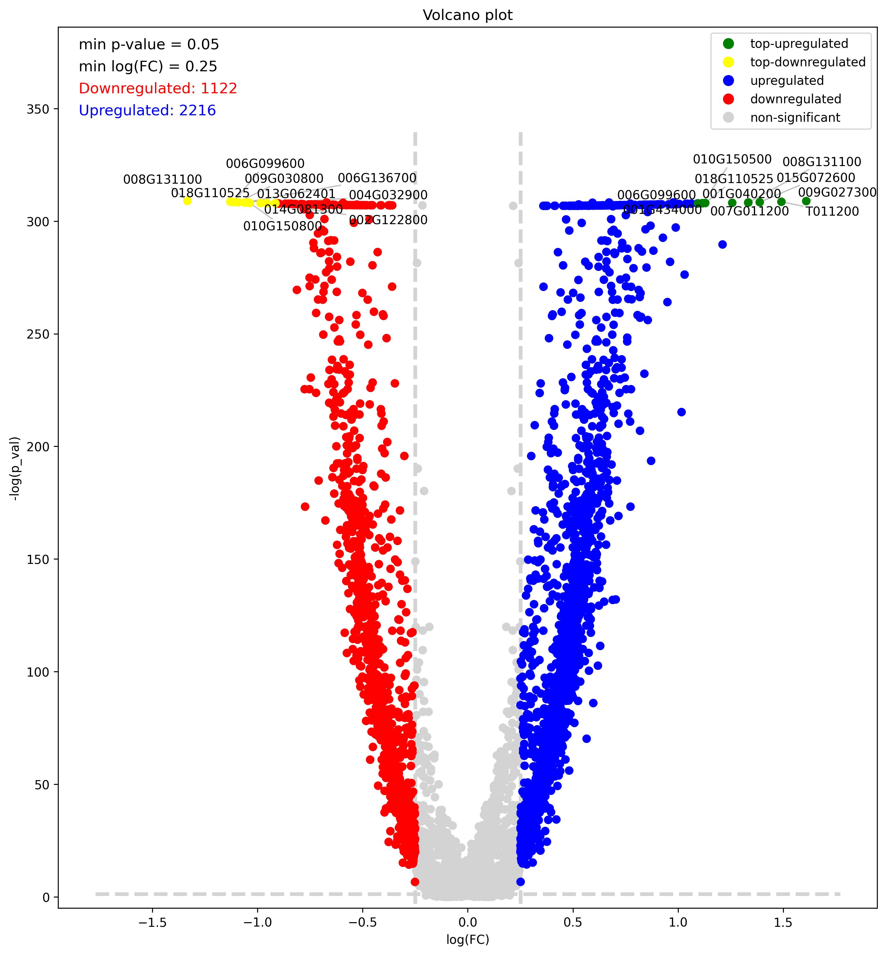
- Volcano plot – Visualization of differentially expressed genes (DEGs) between two groups
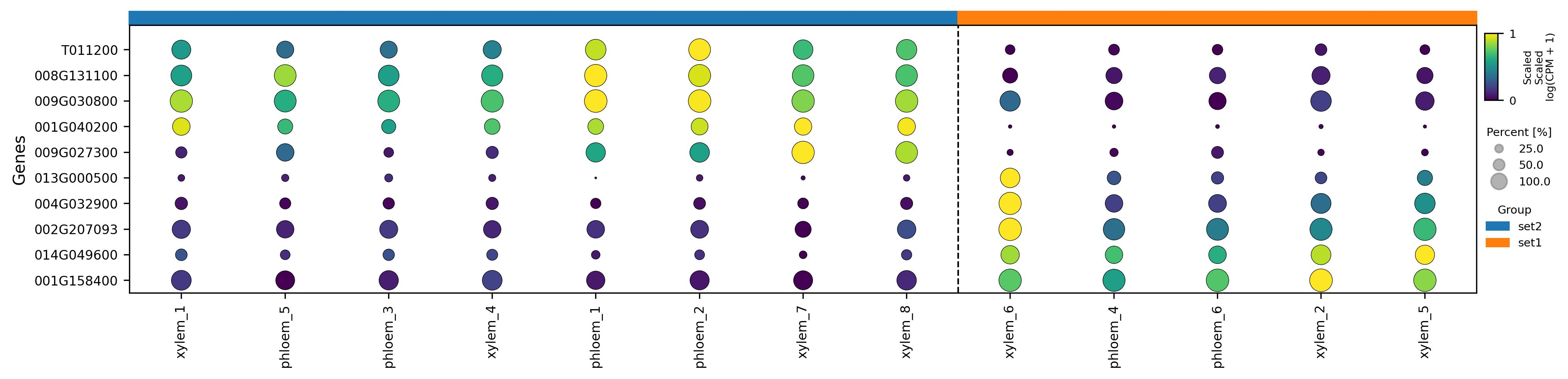
3.33. Dot plot
stats_5 = stats.sort_values(['valid_group', 'esm', 'log(FC)'], ascending=[True, False, False]).groupby('valid_group').head(5)

fig17 = jseq_object.dot_plot(
                 names = None,
                 features = list(set(stats_5['feature'])),
                 name_slot = 'cell_names',
                 scale = True,
                 colors = 'viridis',
                 hclust = 'complete',
                 img_width  = 15,
                 img_high  = 3,
                 label_size = 10,
                 size_scale = 200,
                 y_lab = 'Genes',
                 legend_lab = 'log(CPM + 1)',
                 set_box_size = 5,
                 set_box_high = 0.1,
                 bbox_to_anchor_scale = 25,
                 bbox_to_anchor_perc=(0.90, 0.5),
                 bbox_to_anchor_group=(0.9, 0.3))


fig17.savefig('int_dot_DEG.jpeg', dpi=300, bbox_inches='tight')
3.34. Visualization of feature level on UMAP reduced space
fig18_1 = jseq_object.UMAP_feature(
            feature_name = 'T011200',
            features_data=jseq_object.normalized_data,
            point_size=0.6)

fig18_1.savefig('int_umap_clusters_feature_T011200.jpeg', dpi=300, bbox_inches='tight')
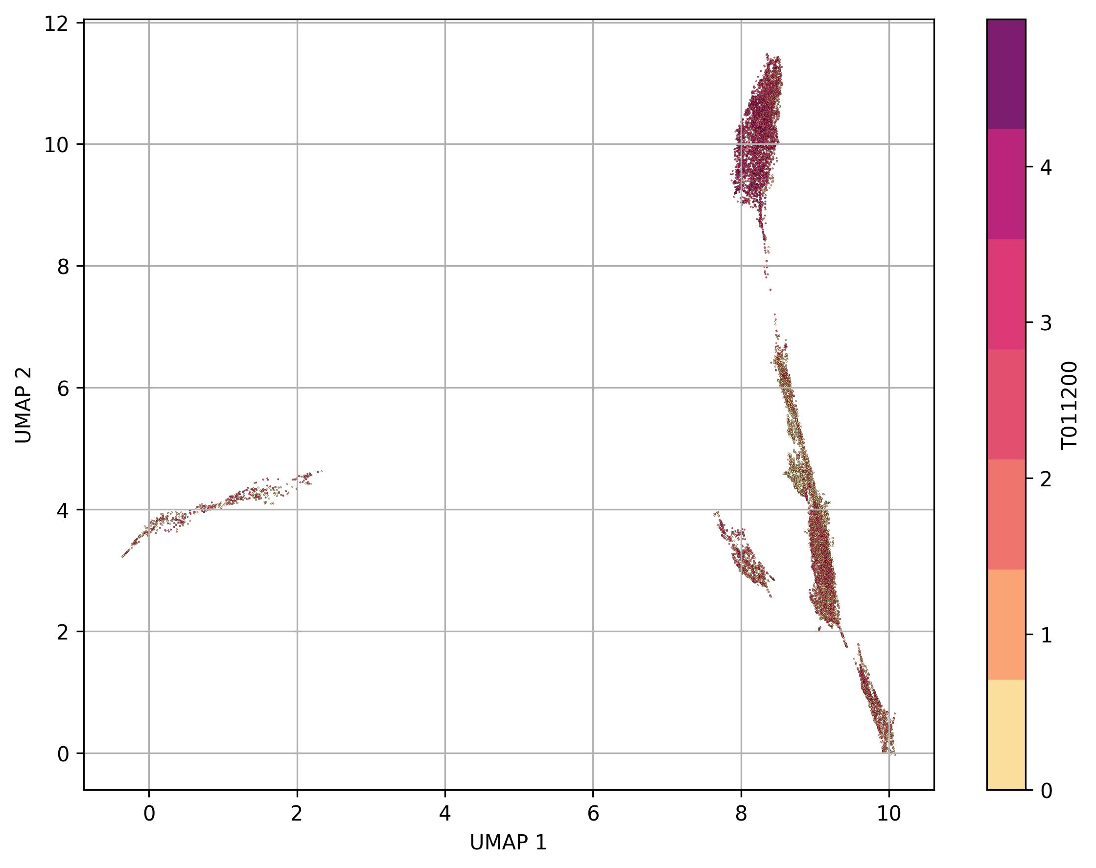
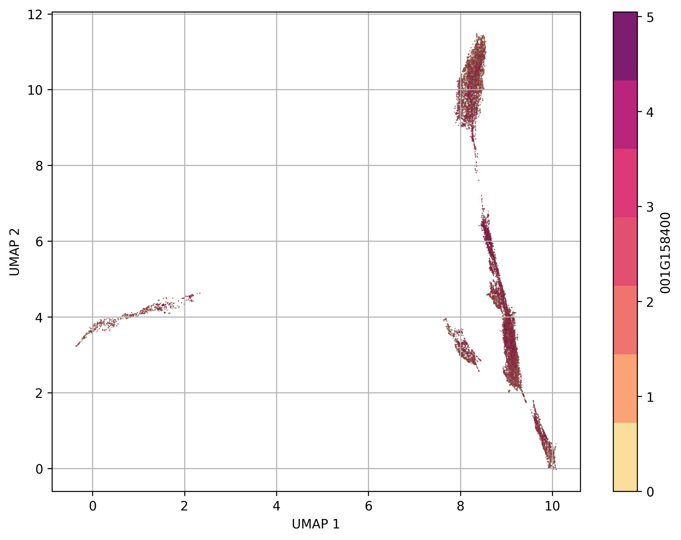
fig18_2 = jseq_object.UMAP_feature(
            feature_name = '001G158400',
            features_data=jseq_object.normalized_data,
            point_size=0.6)

fig18_2.savefig('int_umap_clusters_feature_001G158400.jpeg', dpi=300, bbox_inches='tight')
3.35. Sample / cell composition calculation
import re

jseq_object.data_composition(
                     features_count = list(set([re.sub(r'_.*$', '',x) for x in list(set(jseq_object.input_metadata['cell_names']))])), # get names without numbers for composition calculation
                     name_slot = 'cell_names',
                     set_sep = True
                     )
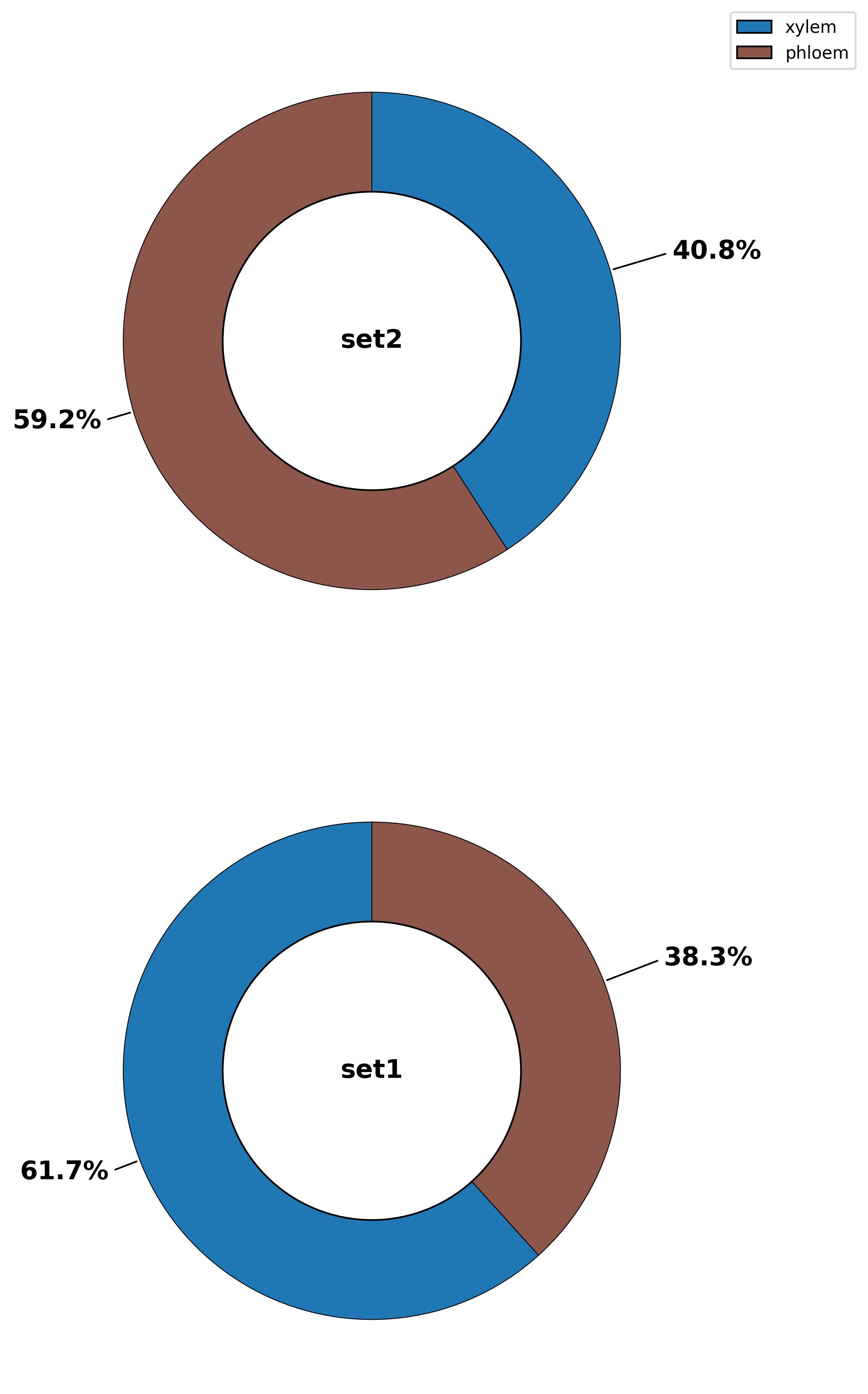
3.36. Composition - pie plot
fig19 = jseq_object.composition_pie(
                    width = 6,
                    height = 6,
                    font_size = 15,
                    cmap  = "tab20",
                    legend_split_col = 1,
                    offset_labels = 0.5,
                    legend_bbox = (1.15, 0.95))


fig19.savefig('int_composition_pie.jpeg', dpi=300, bbox_inches='tight')
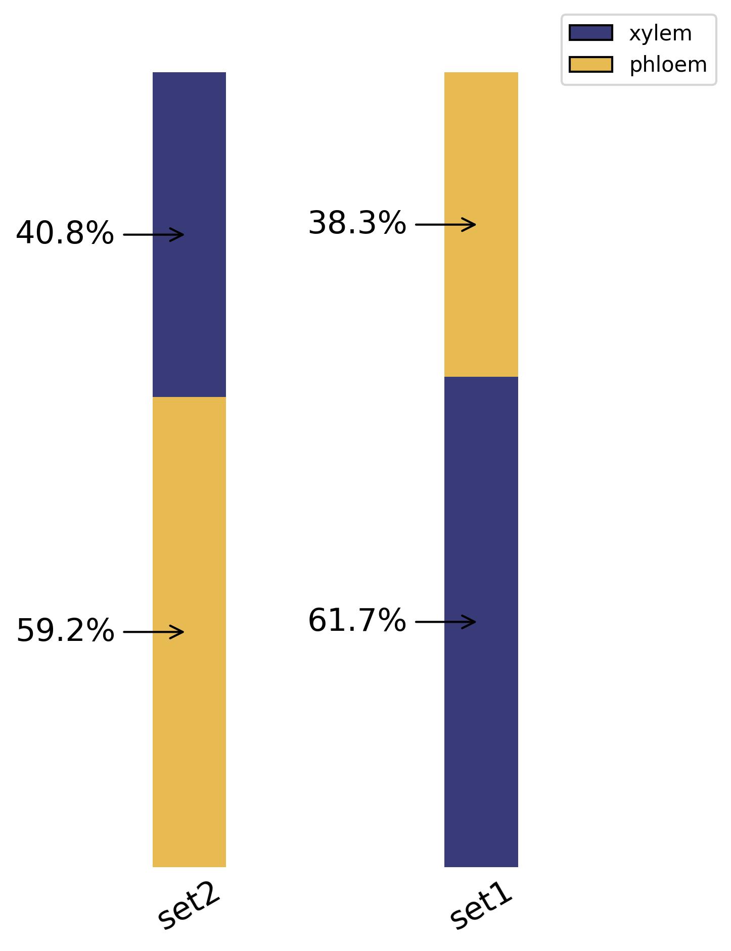
3.37. Composition - bar plot
fig20 = jseq_object.bar_composition(
                    cmap = 'tab20b',
                    width = 2,
                    height = 6,
                    font_size = 15,
                    legend_split_col = 1,
                    legend_bbox = (1.3, 1))


fig20.savefig('int_composition_bar.jpeg', dpi=300, bbox_inches='tight')
3.38. Getting data
met = jseq_object.input_metadata

# full data
data = jseq_object.get_data(set_info=True)

# metadata
metadata = jseq_object.get_metadata()

# partial data
dt = jseq_object.get_partial_data(
                names=['phloem_6'],
                features=['001G000700', '019G047850', '019G089366'],
                name_slot='cell_names')

# more in documentation
3.39. Saving sparse data
# save data from slots in sparse matrix format

jseq_object.save_sparse(
                path_to_save = "data",
                name_slot: str = "cell_names",
                data_slot: str = "normalized",
)
3.40. Saving project
# save whole project with analyses and results

jseq_object.save_project(name = 'tree')
3.41. Loading project
# load project with all attributes & methodes

reoladed_project = COMPsc.load_project('tree.jpkl')
4. Data subclustering
4.1. Loading class
from jdti import COMPsc
4.2. Initialize COMPsc class
import os

jseq_object = COMPsc.project_dir(os.getcwd(), ['set2'])
4.3. Loading data
jseq_object.load_sparse_from_projects(normalized_data=True)
4.4. Select cluster and features for subclustering
jseq_object.calculate_difference_markers()

set(jseq_object.normalized_data.columns)

set_markers = jseq_object.var_data[jseq_object.var_data['valid_group'] == 'xylem / phloem_2 # set2']

set_markers = set_markers.sort_values(['esm', 'log(FC)'], ascending=[False, False]).head(5)
4.5. Prepare subclustering
jseq_object.subcluster_prepare(features = list(set_markers['feature']),
                               cluster='xylem / phloem_2')
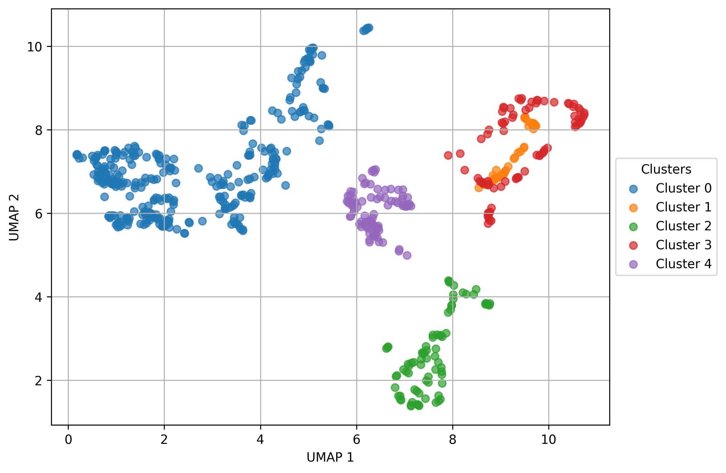
4.6. Define subclusters
fig1 = jseq_object.define_subclusters(
                          umap_num = 5,
                          eps = 1.1,
                          min_samples = 5,
                          n_neighbors = 5,
                          min_dist = 0.1,
                          spread = 1.0,
                          set_op_mix_ratio = 1.0,
                          local_connectivity = 1,
                          repulsion_strength = 1.0,
                          negative_sample_rate = 5,
                          width = 8,
                          height = 6)

fig1.savefig('sub_umap_clust.jpeg', dpi=300, bbox_inches='tight')
4.7. Visualize subclusters features
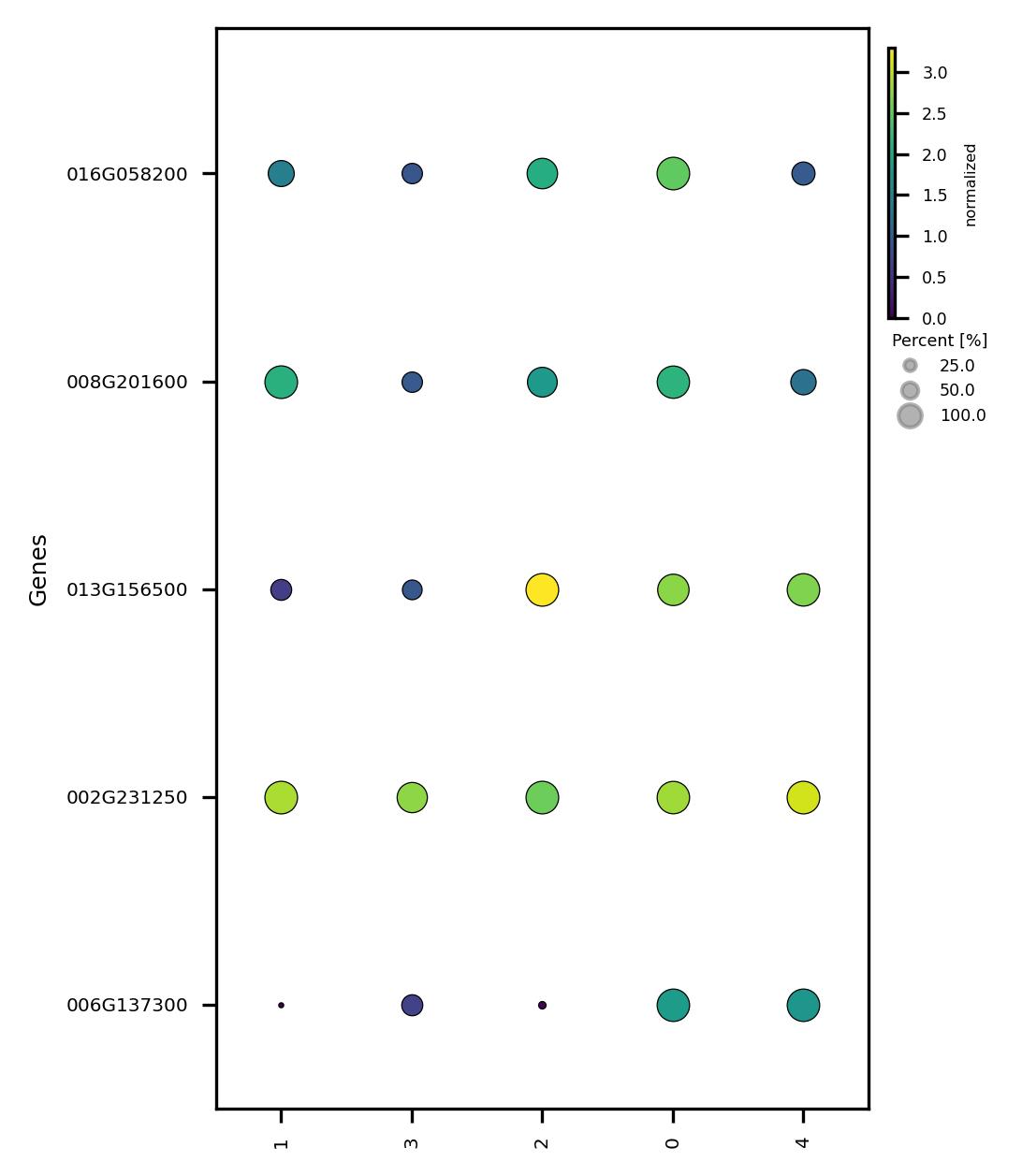
fig2 = jseq_object.subcluster_features_dot(
                                        colors = 'viridis',
                                        hclust = 'complete',
                                        img_width = 3,
                                        img_high = 5,
                                        label_size = 6,
                                        size_scale = 70,
                                        y_lab = 'Genes',
                                        legend_lab = 'normalized')

fig2.savefig('sub_dot_clust_genes.jpeg', dpi=300, bbox_inches='tight')
4.8. Adjust subclusters and check features
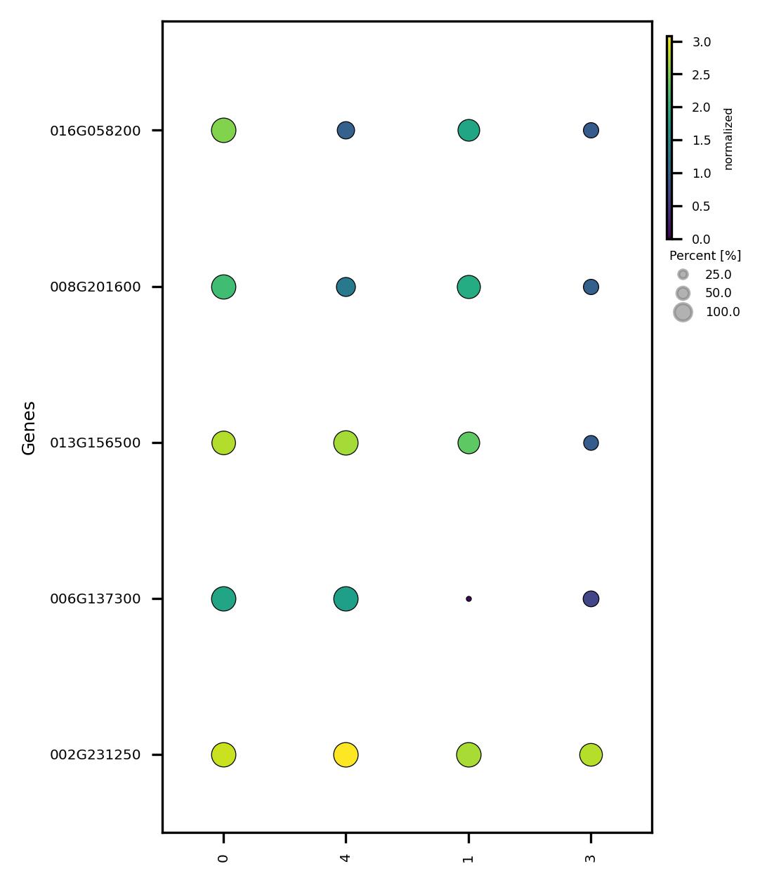
# if subclusters are very similar to each other
# you can use merging subclusters and visualise again

mapping = {
    "old_name": ["1", "2"],
    "new_name": ["1", "1"]
}

jseq_object.rename_subclusters(mapping)
fig3 = jseq_object.subcluster_features_dot(
                                        colors = 'viridis',
                                        hclust = 'complete',
                                        img_width = 3,
                                        img_high = 5,
                                        label_size = 6,
                                        size_scale = 70,
                                        y_lab = 'Genes',
                                        legend_lab = 'normalized')

fig3.savefig('sub_dot_clust_genes_reduced.jpeg', dpi=300, bbox_inches='tight')
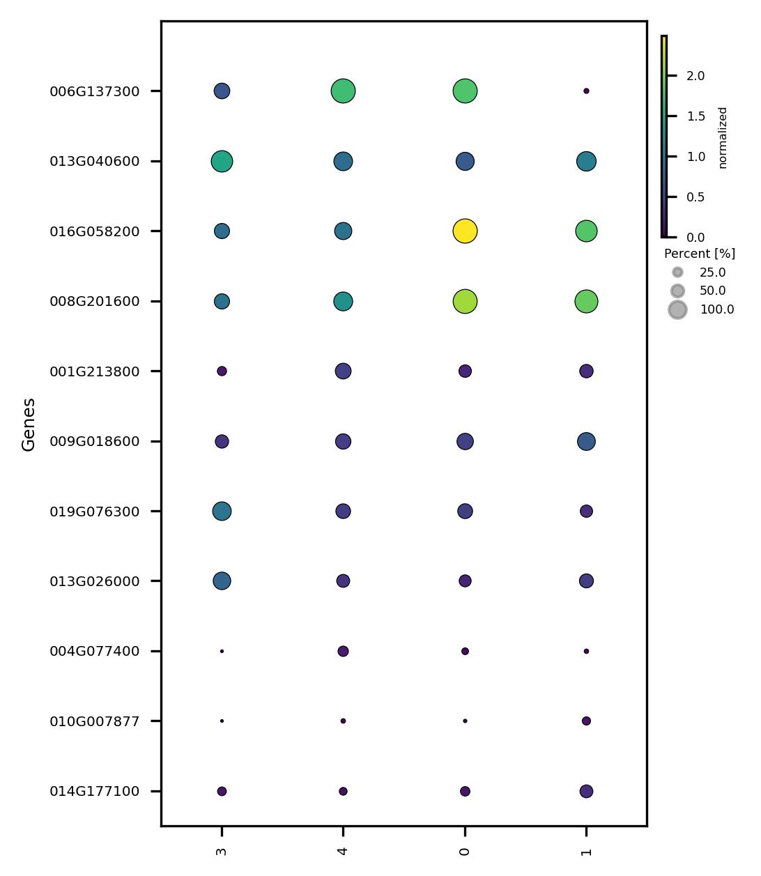
4.9. Calculate DEG for subclusters and visualize
fig4 = jseq_object.subcluster_DEG_dot(
                                    top_n = 3,
                                    min_exp = 0,
                                    min_pct = 0.1,
                                    p_val = 0.05,
                                    colors = 'viridis',
                                    hclust = 'complete',
                                    img_width = 3,
                                    img_high = 5,
                                    label_size = 6,
                                    size_scale = 70,
                                    y_lab = 'Genes',
                                    legend_lab = 'normalized',
                                    n_proc=10)

fig4.savefig('sub_dot_clust_genes_reduced_DEG.jpeg', dpi=300, bbox_inches='tight')
4.10. Confirm subclusters and associate with data
set(jseq_object.input_metadata['cell_names'])
Output before accept:
{'phloem_1', 'phloem_2', 'phloem_3', 'phloem_5', 'xylem / phloem_2',
'xylem / phloem_3', 'xylem_1', 'xylem_4', 'xylem_7', 'xylem_8'}
jseq_object.accept_subclusters()

set(jseq_object.input_metadata['cell_names'])
Output after accept: {'phloem_1', 'phloem_2', 'phloem_3', 'phloem_5', 'xylem / phloem_2.0', 'xylem / phloem_2.1', 'xylem / phloem_2.3', 'xylem / phloem_2.4', 'xylem / phloem_3', 'xylem_1', 'xylem_4', 'xylem_7', 'xylem_8'}
Have fun JBS
1 maintainer

Metadata
1 maintainer
Release files for jdti 0.2.8
For a detailed explanation of source distributions (sdists) and built distributions (wheels), please see the package formats documentation.
Source distribution (sdist)
| File | Size | Uploaded | |
|---|---|---|---|
| jdti-0.2.8.tar.gz | 62.7 kB | Details |
Built distribution (wheel)
| File | Interpreter | ABI | Platform | Reset |
|---|---|---|---|---|
| jdti-0.2.8-py3-none-any.whl | Python 3 | none | any | Details |
Total release size: 120.4 kB
Release files / jdti-0.2.8.tar.gz
| Download URL | jdti-0.2.8.tar.gz |
|---|---|
| Size | 62.7 kB |
| Tags | Source |
|
SHA-256 checksum How to use checksums |
cdd7764c72aedc0780af8225e0ba18fa490f226dcc28ad9d7b5993da924537c3
|
|
BLAKE2b-256 checksum How to use checksums |
2242f83b504da9c51270e4b81111924a8558380108762083a66622135979c98b
|
| Upload date | |
|
Uploaded using Trusted Publishing? What is trusted publishing? |
No |
| Uploaded via |
twine/6.2.0 CPython/3.11.9
|
Release files / jdti-0.2.8-py3-none-any.whl
| Download URL | jdti-0.2.8-py3-none-any.whl |
|---|---|
| Size | 57.7 kB |
| Tags | Python 3 |
|
SHA-256 checksum How to use checksums |
934e761c2ff516af8ea11561de84aa372922d5ee4117e60434168335893e6cc1
|
|
BLAKE2b-256 checksum How to use checksums |
853d1020d63b3d1bcf14100a34fdbe9841d5f4d620f894c1d1babceb62083a79
|
| Upload date | |
|
Uploaded using Trusted Publishing? What is trusted publishing? |
No |
| Uploaded via |
twine/6.2.0 CPython/3.11.9
|














