
jmbayes: JMBayes2 Accelerated Python Implementation
Bayesian joint models for longitudinal and time-to-event data, in Python on the GPU. 10× faster than JMbayes2 with 27× less memory on the largest problem we tested, and the same results. The gap grows with problem size.
| JMbayes2 | jmbayes | |
|---|---|---|
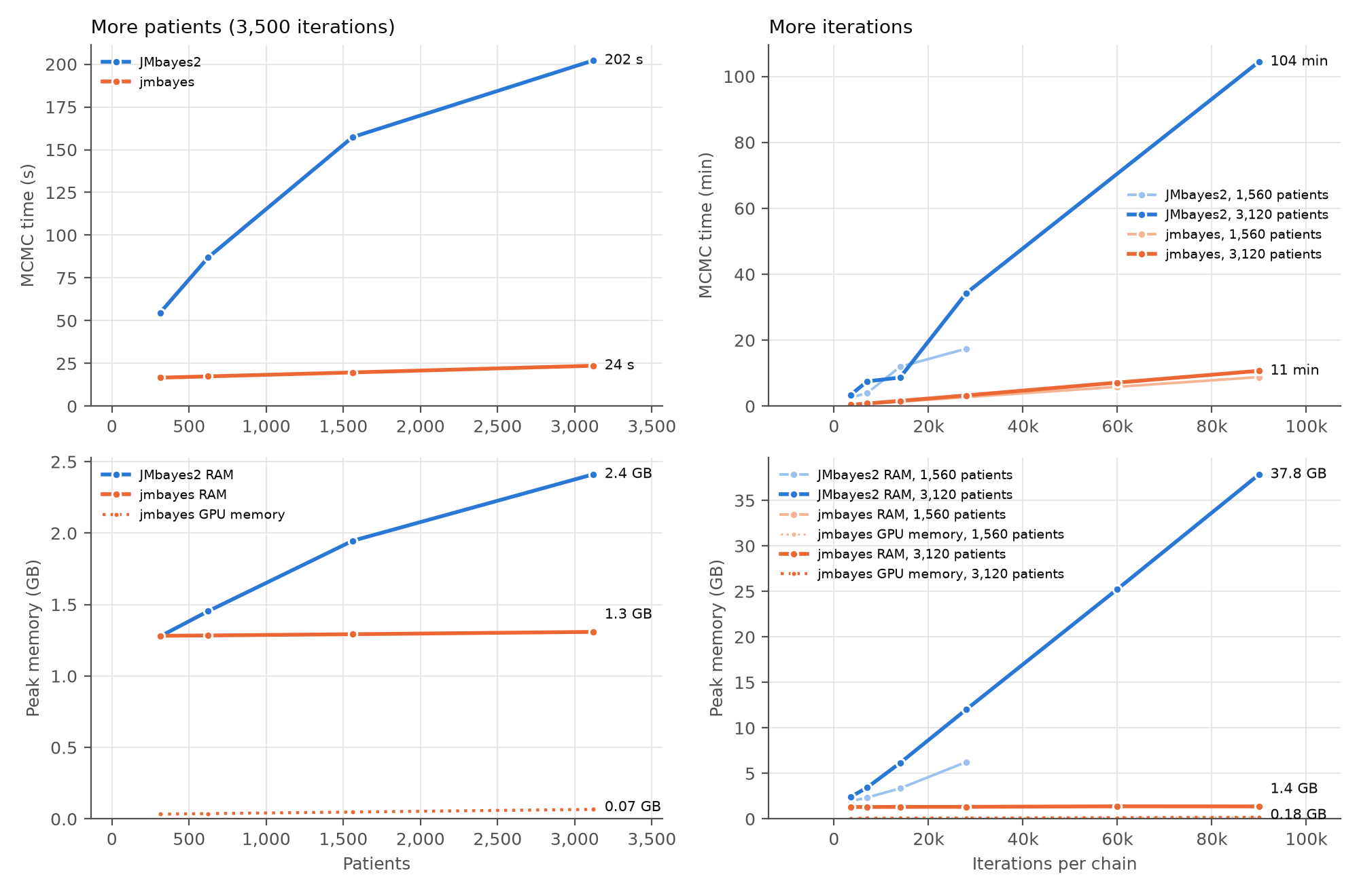
| 3,120 patients, 90,000 iterations | 104 min, 37.8 GB RAM | 11 min, 1.4 GB RAM |
jmbayes is a reimplementation of the R package JMbayes2 by Rizopoulos, Papageorgiou and Miranda Afonso: the same model, the same priors and the same MCMC algorithm.
- Long runs on large cohorts, on ordinary hardware. jmbayes uses 1.3–1.4 GB of RAM and under 0.2 GB of GPU memory in every run we measured, from 3,500 to 90,000 iterations. JMbayes2's memory grows with cohort size × run length: for 3,120 patients it needs 12 GB at 28,000 iterations and 38 GB at 90,000, more than most machines have.
- The bigger the problem, the bigger the gap. 3.3× faster than JMbayes2 on 312 patients, 8–9× on 1,560–3,120 patients at JMbayes2's default run length, and 10× on long runs, still growing at the largest size we tested. With ten times the patients, jmbayes takes 1.4× longer and JMbayes2 3.7× longer (see Benchmarks).
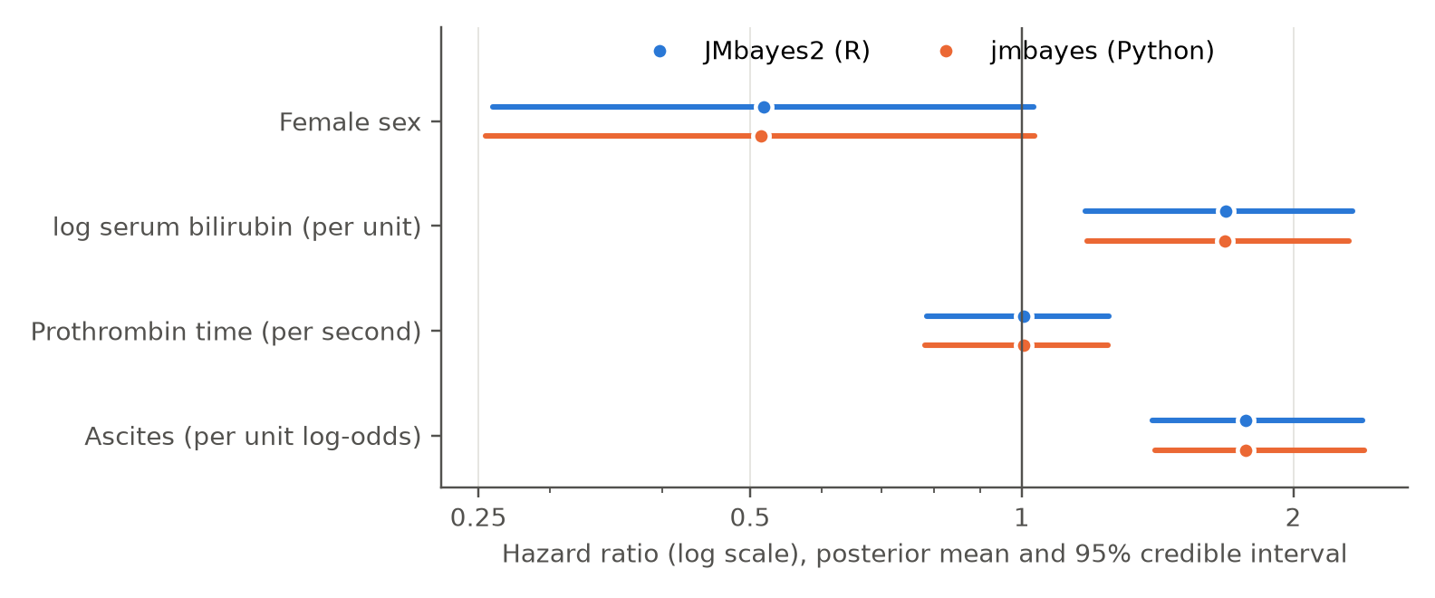
- The same answers, formally tested. In equivalence tests against JMbayes2, all 50 model parameters agree within 0.2 posterior SD and every regression coefficient leads to the same conclusion. jmbayes and JMbayes2 differ from each other no more than two JMbayes2 runs with different seeds do.
- Competing risks and prediction accuracy. Cause-specific hazards as in JMbayes2, and time-dependent AUC, ROC, Brier score and calibration that reproduce JMbayes2's numbers.
- A Python interface, plus JMbayes2-style formula strings if you prefer them.
Install
jmbayes runs on any CPU, and on NVIDIA GPUs through PyTorch. Install PyTorch first, in the version that fits your machine, then this package.
With pip
python -m venv .venv
.venv\Scripts\activate             # macOS/Linux: source .venv/bin/activate
pip install torch                  # see the note below for an NVIDIA GPU on Windows
pip install jmbayes
With conda
conda create -n jmbayes -c conda-forge python=3.11 pytorch numpy scipy pandas statsmodels
conda activate jmbayes
pip install --no-deps jmbayes
From source (for the benchmarks, or to change the code): git clone
https://github.com/neuratom/jmbayes.git, then pip install -e . in that folder.
conda-forge picks a GPU build of PyTorch by itself when it finds an NVIDIA driver.
GPU note. With pip on Linux, pip install torch already includes GPU support. On Windows
it installs the CPU-only build, so use the command that the selector at
pytorch.org/get-started gives for your CUDA
version (run nvidia-smi to see it). Check that the GPU is found:
python -c "import torch; print(torch.cuda.is_available())"
False is fine: everything runs on the CPU, just slower for large studies. Apple GPUs are
not supported yet.
Fit a model
import jmbayes as jmb
from jmbayes import var

visits, patients = jmb.datasets.pbc2()   # example data: visits, and one row per patient
year, sex = var("year"), var("sex")

model = jmb.JointModel(
    event=jmb.Event(time="years", event="status2", covariates=sex),
    markers=[
        jmb.Marker(var("serBilir").log(), fixed=year * sex, random=year),
        jmb.Marker("ascites", fixed=year + sex, random=year, family="binomial"),
    ],
    id="id", time="year",
)
fit = model.fit(visits, patients)
fit.summary()
Benchmarks
The model is the JMbayes2 README model: pbc2, three markers (log serum bilirubin, prothrombin time, ascites), replicated to get more patients. Each run uses 3 chains. JMbayes2 runs its chains in parallel on the CPU; jmbayes ran on the GPU in float32, its default. All runs were on one machine, one run at a time:
| CPU | Intel Core i9-12900K, x86-64 (16 cores: 8 performance + 8 efficiency, 24 threads) |
| RAM | 64 GB |
| GPU | NVIDIA GeForce RTX 3090, 24 GB |
| Software | Windows 11; R 4.6.2 with JMbayes2 0.6-5; Python 3.11, PyTorch 2.6 (CUDA 12.4) |
The two programs agree. Hazard ratios from the same model, fitted by each program (posterior mean and 95% credible interval):
| Patients | Iterations | JMbayes2: MCMC time | JMbayes2: peak RAM | jmbayes: MCMC time | jmbayes: peak RAM | Speed-up |
|---|---|---|---|---|---|---|
| 312 | 3,500 | 55 s | 1.28 GB | 17 s | 1.28 GB | 3.3× |
| 624 | 3,500 | 87 s | 1.45 GB | 17 s | 1.28 GB | 5.0× |
| 1,560 | 3,500 | 157 s | 1.95 GB | 20 s | 1.29 GB | 8.0× |
| 3,120 | 3,500 | 202 s | 2.41 GB | 24 s | 1.31 GB | 8.6× |
| 1,560 | 7,000 | 237 s | 2.34 GB | 41 s | 1.29 GB | 5.8× |
| 1,560 | 14,000 | 716 s | 3.36 GB | 82 s | 1.30 GB | 8.8× |
| 1,560 | 28,000 | 1,046 s | 6.25 GB | 164 s | 1.31 GB | 6.4× |
| 3,120 | 7,000 | 450 s | 3.44 GB | 48 s | 1.31 GB | 9.4× |
| 3,120 | 14,000 | 521 s | 6.15 GB | 96 s | 1.32 GB | 5.4× |
| 3,120 | 28,000 | 2,056 s | 12.0 GB | 196 s | 1.33 GB | 10.5× |
| 3,120 | 60,000 | 5,893 s* | 25.2 GB | 429 s | 1.39 GB | |
| 1,560 | 90,000 | - | - | 529 s | 1.36 GB | |
| 3,120 | 90,000 | 6,266 s | 37.8 GB | 643 s | 1.38 GB | 9.7× |
* This JMbayes2 run overlapped with other work on the machine (98 ms per iteration, against 70–73 ms at 28,000 and 90,000 iterations), so no speed-up is given for it.
The speed comes from the GPU. On the CPU alone, jmbayes is about as fast as JMbayes2 on small cohorts and slower on large ones, with less than half the memory (the CPU runs are in the report).
jmbayes computes in float32 by default; fit(..., dtype="float64") gives 64-bit precision.
The results are statistically the same: both are equivalent to JMbayes2 in the same tests
(float64 report).
The full report, with equivalence tests, hazard ratios, credible intervals, convergence (Rhat) and scaling plots, is in benchmark/jmbayes_vs_JMbayes2.pdf. The scripts that reproduce it are in benchmark/. The R scripts need JMbayes2 installed from CRAN, and are only used for the comparison.
Writing terms
Terms are Python objects and combine with operators:
| You write | Meaning |
|---|---|
year + sex |
main effects |
year * sex |
main effects and their interaction |
year & sex |
the interaction only |
year.ns(2), year.bs(3) |
natural / B-spline of year with 2 / 3 degrees of freedom |
var("serBilir").log() |
log-transformed marker (also .sqrt()) |
Plain column names work too: fixed=["year", "sex", ("year", "sex")] (a tuple is an
interaction), or covariates="sex". The intercept is always included.
Get the results
fit.hazard_ratios()                   # HR, 95% credible interval, P
fit.coefficients("log(serBilir)")     # fixed effects of one marker
fit.random_effects_covariance()       # matrix D
fit.fit_statistics                    # DIC, WAIC, LPML

fit.save("model.jmb")                 # later: fit = jmb.load("model.jmb")
Predict for a patient
new = visits[(visits.id == 93) & (visits.year < 5)].copy()   # measurements up to year 5
new["years"] = 5                                              # event-free up to year 5
new["status2"] = 0

fit.predict(new, times=[5, 6, 7, 8, 10])          # risk of the event by each time
fit.predict(new, process="longitudinal")          # expected marker values
To predict, the patient's random effects are sampled given their data so far. jmbayes
does this step slightly differently from JMbayes2, which we believe weights the
"event-free so far" information inconsistently (details in
NOTES.md). Risks can differ
from JMbayes2's by a few percentage points for some patients (up to 0.07 for PBC
patient 93). fit.predict(..., r_sampling=True) uses JMbayes2's method; given the same
posterior draws, it matches JMbayes2's predictions to within 0.01.
Check how good the predictions are
Using each patient's measurements up to year 5, how well does the model predict who has the event by year 7? Pass data the model has not seen (e.g. a test set) for an honest answer; here the fitting data is used for brevity:
fit.tv_auc(visits, t_start=5, dt=2)        # discrimination: time-dependent AUC
fit.tv_roc(visits, t_start=5, dt=2)        # sensitivity and specificity per cut-off
fit.tv_brier(visits, t_start=5, dt=2)      # Brier score (integrated=True: over years 5-7)
fit.calibration(visits, t_start=5, dt=2)   # ICI, E50, E90; .curve for a calibration plot
These follow JMbayes2's tvAUC(), tvROC(), tvBrier() and calibration_metrics(),
and give the same numbers from the same predicted risks. Patients censored before the
horizon are handled with model-based weights by default (weights="IPCW" for
Kaplan-Meier weights).
Competing risks
When patients can have one of several events, name the value that means censored; every other value of the event column is a cause:
patients["status"] = pd.Categorical(patients["status"], ["alive", "transplanted", "dead"])

model = jmb.JointModel(
    jmb.Event("years", "status", sex, censored="alive"),
    [jmb.Marker(var("serBilir").log(), fixed=year * sex, random=year)],
    id="id", time="year")
fit = model.fit(visits, patients)
fit.hazard_ratios()      # one row per effect and cause, e.g. "sexfemale [dead]"
This is the model JMbayes2 fits with crisk_setup() and strata(CR): each cause has its
own baseline hazard, covariate effects and marker associations. fit.predict(...) gives
each cause's cumulative incidence (column cause). For death and transplantation in PBC,
none of the 50 parameters differed from JMbayes2 in the same equivalence tests, and the
hazard ratios agreed to two decimals
(benchmark/compare_cr.py).
JMbayes2 0.6-5's own predict() fails on this model, so the cumulative incidences were
checked internally: summed over causes they match the overall risk. As in JMbayes2, the
accuracy measures above are for single-event models only.
Your own data
You need two pandas data frames, as in JMbayes2:
- visits (one row per measurement): patient id, visit time, markers, covariates
- patients (one row per patient): the same id, follow-up time, event (0/1), covariates
import pandas as pd
visits = pd.read_csv("visits.csv")
patients = pd.read_csv("patients.csv")
The first category of a text column is the reference group (alphabetical by default). To
choose it: patients["sex"] = pd.Categorical(patients["sex"], ["male", "female"]).
Time can be in any unit (days, months, years) and the column can have any name. Visit times and follow-up times must use the same unit, and effects of time are then per that unit.
The data must be complete: jmbayes does not impute or drop anything for you. The one
exception is an empty marker cell in the visits data, which means that marker was not
measured at that visit (markers are often measured at different visits). Any other missing
value stops the fit with a message naming the columns and the number of rows, as does
invalid data (e.g. log of values <= 0, an event column not coded 0/1, or a patient in
only one of the two tables).
Options
jmb.Marker("y", fixed=year + var("age"))                      # random intercept only
jmb.Marker("y", fixed=year, random=year, uncorrelated=True)   # independent random effects
jmb.Marker("y", fixed=year, random=year,
           association=["value", "slope"])           # current value, slope and/or "area"

jmb.JointModel(..., independent="all")               # markers independent of each other

model.fit(visits, patients,
          n_iter=12000, n_burnin=2000, n_thin=5,     # MCMC length (default 3500 / 500 / 1)
          n_chains=3,                                # more chains are cheap on a GPU
          device="cpu",                              # default: GPU if available
          save_loglik=True)                          # keep the per-patient table (below)
DIC, WAIC and LPML are always computed, from running totals, so jmbayes does not need to
keep each patient's log-likelihood at every iteration (the table that makes JMbayes2's
memory grow). If you want that table, for example for PSIS-LOO with its Pareto-k
diagnostic, pass save_loglik=True: fit.loglik is then an array of
chains × iterations × patients (patients in the order of fit.patient_ids). It takes
(iterations − burn-in) × chains × patients numbers of memory, e.g. 2.2 GB for 2,000 patients,
3 chains and 90,000 iterations.
Check convergence in fit.survival_table(): Rhat should be below about 1.05. If not,
run longer or with more chains.
Not supported yet (you get a clear error): outcome families other than gaussian and binomial, strata other than competing risks, left truncation, interval censoring.
Prefer R formulas?
You can also write the same model with JMbayes2-style formula strings. Both interfaces build the same objects underneath and give identical results:
fit = jmb.jm(
    jmb.Survival("Surv(years, status2) ~ sex", data=patients),
    [jmb.Longitudinal("log(serBilir) ~ year * sex", random="~ year | id"),
     jmb.Longitudinal("ascites ~ year + sex", random="~ year | id", family="binomial")],
    data=visits, time_var="year",
    functional_forms="~ value(log(serBilir)) + slope(log(serBilir))")
How it works
The MCMC is the same Metropolis-within-Gibbs sampler as JMbayes2: the same update order, proposals, adaptive tuning and priors. What changes is how it runs:
- The chains run as one batch on the GPU (or on CPU threads).
- Each iteration is recorded once as a CUDA graph and then replayed.
- The fit statistics (DIC, WAIC, LPML) are accumulated as the run goes, so the per-draw log-likelihood table is never stored. That table is what makes JMbayes2's memory grow.
Implementation notes, including places where we found JMbayes2's behaviour questionable, are in NOTES.md.
Citation
If you use jmbayes, please also cite JMbayes2: Rizopoulos D, Papageorgiou G, Miranda Afonso P. JMbayes2: Extended Joint Models for Longitudinal and Time-to-Event Data. R package, https://github.com/drizopoulos/JMbayes2.
jmbayes is an independent reimplementation. It is not affiliated with or endorsed by the authors of the R packages JMbayes and JMbayes2.
Licence
GPL-3.0-or-later, like JMbayes2, from which this is derived.
1 maintainer

Metadata
1 maintainer
Release files for jmbayes 0.5.1
For a detailed explanation of source distributions (sdists) and built distributions (wheels), please see the package formats documentation.
Source distribution (sdist)
| File | Size | Uploaded | Provenance | Actions |
|---|---|---|---|---|
| jmbayes-0.5.1.tar.gz | 160.2 kB | Without provenance | Details for jmbayes-0.5.1.tar.gz |
Built distribution (wheel)
| File | Interpreter | ABI | Platform | Actions Reset |
|---|---|---|---|---|
| jmbayes-0.5.1-py3-none-any.whl | Python 3 | none | any | Details for jmbayes-0.5.1-py3-none-any.whl |
Total release size: 308.2 kB
Release files / jmbayes-0.5.1.tar.gz
| Download URL | jmbayes-0.5.1.tar.gz |
|---|---|
| Size | 160.2 kB |
| Tags | Source |
|
SHA-256 checksum How to use checksums |
c74bfd53217c8ff6212bb69639ecbfd5c35f9fe4382a28e59f9bff158cc3db74
|
|
BLAKE2b-256 checksum How to use checksums |
f0f0ac36d6e3449635e7cb0b1f7fb97ea97397a141c9724c340da04aa5700322
|
| Upload date | |
|
Uploaded using Trusted Publishing? What is trusted publishing? |
No |
| Uploaded via |
twine/7.0.0 CPython/3.11.2
|
Release files / jmbayes-0.5.1-py3-none-any.whl
| Download URL | jmbayes-0.5.1-py3-none-any.whl |
|---|---|
| Size | 148.0 kB |
| Tags | Python 3 |
|
SHA-256 checksum How to use checksums |
dd259470a26af49df6071ad69205232c7cd68f680d32207a66a79acb4f3865fc
|
|
BLAKE2b-256 checksum How to use checksums |
e34099d792846069fb7f729e78ba564a5867c0dd29a5623c55c0b1229a261b06
|
| Upload date | |
|
Uploaded using Trusted Publishing? What is trusted publishing? |
No |
| Uploaded via |
twine/7.0.0 CPython/3.11.2
|
Security for jmbayes 0.5.1
Provenance
Provenance describes where a file came from. On PyPI, provenance is shared via attestations, which provide a verifiable record of the build or publishing details. View details, limitations and caveats.
No provenance found
None of the files in this release were uploaded with provenance metadata.
A note on package security
PyPI is a repository for distributing packages, not a service for auditing them. While third-party security researchers and our staff do their best to detect and remove malicious packages, PyPI cannot guarantee the quality, security or suitability of any given package.
To learn more about protecting yourself from malicious actors, visit our package security documentation.














