Reservoir simulation with JutulDarcy in Python.

Project description
PyJutulDarcy
Python wrapper for JutulDarcy.jl, a fully differentiable reservoir simulator written in Julia. Key features:
- Immiscible, black-oil and compositional multiphase flow
- Geothermal simulation and simulation of CO2 sequestration
- Can read standard input files and corner-point grids, or make your own
This package facilitates automatic installation of JutulDarcy from Python, as well as a minimal interface that allows fast simulation of .DATA files in pure Python. For more details about JutulDarcy.jl, please see the Julia Documentation. If you want to run MPI or CUDA accelerated simulations we recommend working either in Julia or the standalone compiled version.
The package also provides access to all the functions of the Julia version under jutuldarcy.jl.JutulDarcy, jutuldarcy.jl.GeoEnergyIO and jutuldarcy.jl.Jutul. These functions are directly wrapped using JuliaCall. For more details, see the JuliaCall Documentation on converting of types.
Installation
The package can be installed with pip:
pip install jutuldarcy
On first time usage of the package JuliaCall will automatically install Julia and manage all dependency packages.
Activating plotting
There is highly experimental support for 3D and 2D visualization. To enable, you can either add GLMakie to your environment manually, or run the following:
import jutuldarcy as jd
jd.install_plotting()
Note that this requires that you are running in an environment that supports plotting (OpenGL capable, i.e. not at a SSH remote without forwarding).
Examples
Copies of these examples can be found in the examples directory.
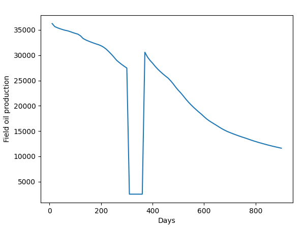
A minimal example: Running a benchmark file
import jutuldarcy as jd
# Load SPE9 dataset to disk
pth = jd.test_file_path("SPE9", "SPE9.DATA")
# Simulate the model and convert to Python dicts
res = jd.simulate_data_file(pth, convert = True)
# Get field quantities and plot
import matplotlib.pyplot as plt
fopr = res["FIELD"]["FOPR"]
days = res["DAYS"]
plt.plot(days, fopr)
plt.ylabel("Field oil production")
plt.xlabel("Days")
plt.show()
Here, res is a standard dict containing the following fields:
- "FIELD": Field quantities (average pressure, total water injection, etc) as numpy arrays.
- "WELLS": Well quantities (bottom hole pressures, injection rates, production rates, etc)
- "STATES": Reservoir states for all active cells, given as a list with a dict for each timestep. For example,
res["STATES"][10]["Rs"]will give you an array of the solution gas-oil-ratio at step 10. - "DAYS": Array of the number of days elapsed for each step.
Optionally, if the keyword argument convert to simulate_data_file is set to False or left defaulted, the "full" output as seen in Julia will be returned, where it is possible to get access to grid geometry, model parameters, and so on.
Setting up a simulation without input file
This example is a port of the first JutulDarcy.jl documentation example. If you want to understand a bit more about what is going on, please refer to that page.
Note that only a subset of the full set of routines are available directly in the wrapper. PRs that add more wrapping functionality is welcome.
import jutuldarcy as jd
import numpy as np
# Grab some unit conversion factors
day = jd.si_unit("day")
Darcy = jd.si_unit("darcy")
kg = jd.si_unit("kilogram")
meter = jd.si_unit("meter")
bar = jd.si_unit("bar")
# Set up mesh
nx = ny = 25
nz = 10
cart_dims = (nx, ny, nz)
physical_dims = (1000.0*meter, 1000.0*meter, 100.0*meter)
g = jd.CartesianMesh(cart_dims, physical_dims)
# Convert to unstructured representation
g = jd.UnstructuredMesh(g)
domain = jd.reservoir_domain(g, permeability = 0.3*Darcy, porosity = 0.2)
Injector = jd.setup_vertical_well(domain, 1, 1, name = "Injector")
Producer = jd.setup_well(domain, (nx, ny, 1), name = "Producer")
# Show the properties in the domain
phases = (jd.LiquidPhase(), jd.VaporPhase())
rhoLS = 1000.0*kg/meter**3
rhoGS = 100.0*kg/meter**3
reference_densities = [rhoLS, rhoGS]
sys = jd.ImmiscibleSystem(phases, reference_densities = reference_densities)
model = jd.setup_reservoir_model(domain, sys, wells = [Injector, Producer])
# Replace dynamic functions with custom ones
c = np.array([1e-6/bar, 1e-4/bar])
density = jd.jl.ConstantCompressibilityDensities(
    p_ref = 100*bar,
    density_ref = reference_densities,
    compressibility = c
)
kr = jd.jl.BrooksCoreyRelativePermeabilities(sys, np.array([2.0, 3.0]))
jd.replace_variables(model, PhaseMassDensities = density, RelativePermeabilities = kr)
# Set the initial conditions
state0 = jd.setup_reservoir_state(model,
    Pressure = 120*bar,
    Saturations = np.array([1.0, 0.0])
)
# Set up reporting steps
nstep = 25
dt = np.repeat(365.0*day, nstep)
# Set up timestepping and well controls
pv = jd.pore_volume(model, parameters)
inj_rate = 1.5*np.sum(pv)/sum(dt)
I_ctrl = jd.setup_injector_control(inj_rate, "rate", np.array([0.0, 1.0]), density = rhoGS)
P_ctrl = jd.setup_producer_control(100*bar, "bhp")
controls = dict(Injector = I_ctrl, Producer = P_ctrl)
forces = jd.setup_reservoir_forces(model, control = controls)
result = jd.simulate_reservoir(state0, model, dt, parameters = parameters, forces = forces)
Converting to Python dict
We can convert the result into a standard dict with numpy array types:
case = jd.setup_jutul_case(state0, model, dt, forces, parameters)
res_py = jd.convert_to_pydict(result, case, units = "field")
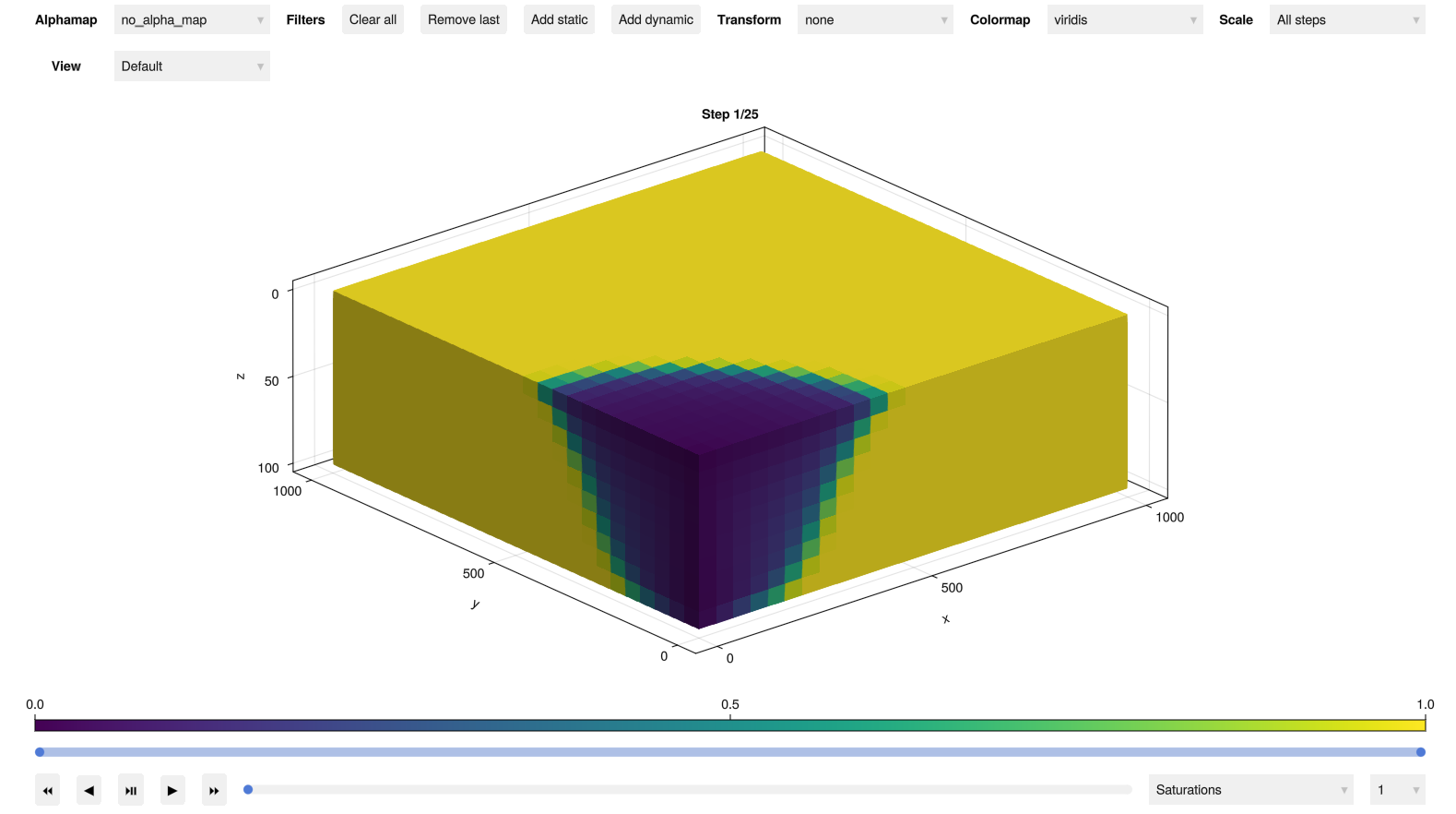
Plotting results (experimental)
We can also plot the results if the plotting has been installed:
plt = jd.plot_reservoir(model, result.states)
jd.make_interactive()
Paper and citing
The main paper describing JutulDarcy.jl is JutulDarcy.jl - a Fully Differentiable High-Performance Reservoir Simulator Based on Automatic Differentiation, available as open access from Springer:
@article{jutuldarcy,
  title={JutulDarcy.jl - a fully differentiable high-performance reservoir simulator based on automatic differentiation},
  author={M{\o}yner, Olav},
  journal={Computational Geosciences},
  volume={29},
  number={30},
  year={2025},
  publisher={Springer}
}
Contributing
Contributions that expose additional functionality is welcome.


Download files
Download the file for your platform. If you're not sure which to choose, learn more about installing packages.
Source Distribution
Built Distribution
Filter files by name, interpreter, ABI, and platform.
If you're not sure about the file name format, learn more about wheel file names.
Copy a direct link to the current filters
File details
Details for the file jutuldarcy-1.2.1.tar.gz.
File metadata
- Download URL: jutuldarcy-1.2.1.tar.gz
- Upload date:
- Size: 15.0 kB
- Tags: Source
- Uploaded using Trusted Publishing? No
- Uploaded via: twine/6.2.0 CPython/3.14.3
File hashes
| Algorithm | Hash digest | |
|---|---|---|
| SHA256 |
e3ada04ceec223c1497f05d58e25223ae54410f1c2917becd67132001e5b94af
|
|
| MD5 |
36f4bf3f612ee0d8532bf2c1500e2bfb
|
|
| BLAKE2b-256 |
1fc73af8f2c1c03387e0e74d98b879e845c4df7831eb7c74eee52326081d0384
|
File details
Details for the file jutuldarcy-1.2.1-py3-none-any.whl.
File metadata
- Download URL: jutuldarcy-1.2.1-py3-none-any.whl
- Upload date:
- Size: 13.3 kB
- Tags: Python 3
- Uploaded using Trusted Publishing? No
- Uploaded via: twine/6.2.0 CPython/3.14.3
File hashes
| Algorithm | Hash digest | |
|---|---|---|
| SHA256 |
dcb1c55068a882330ffd8331c24b3f749a21e5d6fe45c4c9d3b47ae75fc19f90
|
|
| MD5 |
569215fa9402cafe196355bf68f7df07
|
|
| BLAKE2b-256 |
fc807cff6457a4935edad0d7c110db49877f32676cfb8e7a25b87b3c72414e71
|


