
Kalman filter with EM parameter estimation for time series forecasting
Verified details
These details have been verified by PyPIProject links
GitHub Statistics
Maintainers

Project description
Kalman-EM Time Series Forecaster




A production-ready time series forecasting framework based on the Kalman filter with parameters learned by the Expectation-Maximisation (EM) algorithm, packaged as an interactive Streamlit application.
Table of contents
- Overview
- Mathematical background
- Architecture
- Installation
- Streamlit application
- Command-line examples
- Python API
- Datasets
- Results
- Documentation
- Project structure
Overview
This project implements a Linear Gaussian State-Space model whose parameters are estimated from data via the EM algorithm (Expectation-Maximisation). The framework handles:
- Univariate and multivariate time series
- Missing observations (NaN-aware Kalman filter)
- Strongly seasonal series via an optional STL pre-decomposition pipeline
- Honest backtesting with one-step-ahead predictions
- Multi-step forecasting with calibrated uncertainty intervals
- Multiple random restarts to escape local optima
Five real-world domains are demonstrated out-of-the-box:
| Domain | Dataset | MAE | MAPE | Coverage ±2σ |
|---|---|---|---|---|
| Finance | Apple stock (AAPL, 2022–2024) | 2.52 USD | 1.13 % | 93 % |
| Energy | French electricity (RTE, 2020–2024) | 2 337 MW | 4.81 % | 98 % |
| Transport | SNCF TGV punctuality (2018–2025) | 1.74 pp | 1.96 % | 100 % |
| Meteorology | Paris daily temperature (2020–2024) | 1.59 °C | — | 95 % |
| Astronomy | Monthly sunspot number (1749–2026) | 15.60 | — | 96 % |
Mathematical background
State-space model
x_t = F x_{t-1} + w_t,   w_t ~ N(0, Q)   (state equation)
y_t = H x_t    + v_t,   v_t ~ N(0, R)   (observation equation)
x_0 ~ N(μ₀, Σ₀)
| Symbol | Shape | Role |
|---|---|---|
x_t |
(d,) |
Latent state — e.g. level + trend |
y_t |
(m,) |
Observed time series |
F |
(d, d) |
State transition matrix |
H |
(m, d) |
Observation matrix |
Q |
(d, d) |
Process noise covariance |
R |
(m, m) |
Observation noise covariance |
EM algorithm
All six parameters {F, H, Q, R, μ₀, Σ₀} are learned end-to-end from data.
E-step — run the Kalman filter (forward) and RTS smoother (backward) to compute sufficient statistics:
E[x_t | Y], E[x_t xₜᵀ | Y], E[x_t x_{t-1}ᵀ | Y]
M-step — closed-form updates (solved via Cholesky decomposition for numerical stability):
F  ← (Σ_t E[x_t x_{t-1}ᵀ]) (Σ_t E[x_{t-1} x_{t-1}ᵀ])⁻¹
Q  ← (1/T) Σ_t (E[x_t xₜᵀ] − F E[x_t x_{t-1}ᵀ]ᵀ)
H  ← (Σ_t y_t E[xₜᵀ]) (Σ_t E[x_t xₜᵀ])⁻¹
R  ← (1/T) Σ_t (y_t yₜᵀ − H y_t E[xₜᵀ]ᵀ)
Convergence is checked with a relative criterion: ΔLL / (1 + |LL|) < tol, which is scale-invariant and more reliable than an absolute threshold.
Numerical robustness
The implementation uses several techniques for numerical stability:
| Technique | Where | Benefit |
|---|---|---|
Cholesky + solve |
Kalman gain, M-step F/H | Avoids explicit matrix inversion |
| Log-det via Cholesky diagonal | Log-likelihood | No sign ambiguity |
| Mahalanobis via triangular solve | Log-likelihood | Numerically stable |
Joseph form (I−KH)P(I−KH)ᵀ + KRKᵀ |
Filter update | Preserves PSD of Σ |
| Cholesky-first PD enforcement | All covariances | Fast path; eigh only on failure |
| Spectral radius clipping ρ(F) ≤ 0.9999 | M-step | Prevents explosive dynamics |
STL + Kalman-EM pipeline (for seasonal series)
When the series exhibits strong seasonality, a pre-decomposition step is applied before fitting:
Raw series
    │
    ▼
STL decomposition  (Seasonal-Trend via Loess)
    ├── trend      →  linear extrapolation
    ├── seasonal   →  day-of-year / month profile
    └── residual   →  fed to Kalman-EM
                           │
                           ▼
                      Kalman-EM fit
                           │
                           ▼
                   Recomposition: ŷ = ŷ_residual + seasonal + trend
This reduces residual variance to ~16 % of total variance and cuts MAPE by 60 %.
Architecture
kalman_em/
├── kalman_filter.py   Kalman filter + RTS smoother (Cholesky, Joseph form, NaN-aware)
├── em.py              EM algorithm — E-step / M-step, n_restarts, relative convergence
├── model.py           KalmanEM public API  (fit / filter / smooth / forecast)
└── __init__.py

examples/
├── evaluate.py             Generic one-step-ahead backtest (all datasets via --col)
├── stock_prediction.py     AAPL price smoothing + 30-day forecast
├── energy_prediction.py    French electricity: STL + Kalman-EM
├── transport_prediction.py SNCF TGV traffic: STL + Kalman-EM
└── sunspot_prediction.py   Solar cycle backtest (1749–2026)

data/
├── AAPL_prices.csv             752 trading days (2022–2024)
├── france_conso_elec.csv       1 827 daily observations (2020–2024)
├── sncf_tgv_mensuel.csv        96 monthly observations (2018–2025)
├── paris_temperature_daily.csv 1 827 daily observations (2020–2024)
├── sunspots_monthly.csv        3 326 monthly observations (1749–2026)
└── README.md                   Data provenance and column descriptions

assets/                      Backtest result figures
docs/
├── kalman_em_theory.pdf     Full theoretical derivations (Kalman + EM)
└── numerical_issues.md      Numerical pitfalls and best practices

app.py                       Streamlit Forecaster application
requirements.txt
Installation
# 1. Clone the repository
git clone https://github.com/MarouaneAEF/kalman_time_series.git
cd kalman_time_series

# 2. Create a virtual environment (recommended)
python -m venv .venv
source .venv/bin/activate        # Windows: .venv\Scripts\activate

# 3. Install dependencies
pip install -r requirements.txt
Or install the core library from PyPI:
pip install kalman-em                    # core only (numpy + scipy)
pip install "kalman-em[app]"             # + streamlit, matplotlib, pandas, statsmodels
Dependencies:
| Package | Version | Purpose |
|---|---|---|
numpy |
≥ 1.24 | Matrix operations, Cholesky decomposition |
scipy |
≥ 1.10 | Eigenvalue computation |
pandas |
≥ 2.0 | Data loading and date handling |
matplotlib |
≥ 3.7 | Visualisation |
statsmodels |
≥ 0.14 | STL decomposition |
streamlit |
≥ 1.32 | Interactive web application |
Streamlit application
The Forecaster app provides a no-code interface to the entire pipeline.
Launch
streamlit run app.py
The app opens in your browser at http://localhost:8501.
Workflow
1. Upload any CSV  →  date column + numeric value column
2. Configure preprocessing (STL period auto-detected)
3. Set model hyperparameters  →  Run Analysis
4. Explore the 4 result tabs
Sidebar controls
| Control | Description |
|---|---|
| Upload CSV | Any CSV with a date column and a numeric value column |
| Date column | Automatically guessed; can be overridden |
| Value column | All numeric columns are listed |
| Remove seasonality (STL) | Toggle STL pre-decomposition |
| STL period | Auto-detected from data frequency (daily→365, monthly→12, …) |
| Latent dimension d | Size of hidden state vector (1–6; default 2 = level + trend) |
| Max EM iterations | 20–500 (default 200) |
| Test set ratio | Fraction held out for backtesting (default 20 %) |
| Convergence tolerance | Relative criterion ΔLL/(1+|LL|) (default 1e-5) |
| Random restarts | 1–5 EM runs with different initialisations; best log-lik kept |
| Run Analysis | Triggers the full pipeline |
Result tabs
📊 Raw Data
Plot of the uploaded series and a data preview table.
🔧 Preprocessing
If STL is enabled: four-panel decomposition (observed / trend / seasonal / residual) and the residual variance ratio — a measure of how much structure STL captured.
📈 Backtest
One-step-ahead prediction results on the held-out test set.
| Metric | Description |
|---|---|
| MAE | Mean Absolute Error |
| RMSE | Root Mean Squared Error |
| MAPE (%) | Mean Absolute Percentage Error |
| Coverage ±2σ (%) | Fraction of actuals inside the ±2σ prediction band (target ≈ 95 %) |
Three-panel figure:
- Actual vs predicted with ±2σ confidence band
- Absolute error per time step
- Normalised residuals (should follow N(0,1) for a well-fitted model)
🔬 Model Parameters
Learned state-space matrices displayed as annotated heatmaps (F, H, Q, R, Σ₀), EM convergence curve, spectral radius ρ(F), and restart summary.
Tips for best results
- Finance / smooth signals: disable STL, use
d=2. - Daily data with annual cycle (energy, weather): enable STL with
period=365. - Monthly data (transport, sales): enable STL with
period=12. - Quasi-periodic signals (sunspots): disable STL, use
d=4. - Coverage ≈ 95 % is the calibration target for ±2σ intervals. If coverage is lower, increase
d. - Use Random restarts ≥ 3 on short or noisy series to avoid local optima.
Command-line examples
Generic backtest (any dataset)
# AAPL stock
python examples/evaluate.py --csv data/AAPL_prices.csv --col Close --latent 2

# French electricity consumption
python examples/evaluate.py --csv data/france_conso_elec.csv --col Conso_MW --latent 4

# Paris daily temperature
python examples/evaluate.py --csv data/paris_temperature_daily.csv --col Temp_C --latent 4

# SNCF TGV punctuality
python examples/evaluate.py --csv data/sncf_tgv_mensuel.csv --col ponctualite_pct --latent 2

# Solar cycle (sunspots)
python examples/evaluate.py --csv data/sunspots_monthly.csv --col Sunspots --latent 4 --test_ratio 0.15
Dedicated scripts
# Stock forecast (30 days ahead)
python examples/stock_prediction.py --csv data/AAPL_prices.csv --days 30

# Electricity: STL + Kalman-EM
python examples/energy_prediction.py --csv data/france_conso_elec.csv --days 30

# SNCF TGV traffic
python examples/transport_prediction.py --csv data/sncf_tgv_mensuel.csv --target trains_prevus

# Sunspot one-step-ahead backtest
python examples/sunspot_prediction.py --test_ratio 0.15 --latent 4
Python API
import numpy as np
from kalman_em import KalmanEM

# Y: (T, m) array — observations (NaN allowed for missing values)
Y = prices.reshape(-1, 1)

# --- Fit ---
model = KalmanEM(
    d=2,            # latent state dimension
    n_iter=200,     # max EM iterations
    tol=1e-5,       # relative convergence tolerance
    diagonal_R=True,
    n_restarts=3,   # run EM 3 times, keep best log-likelihood
    verbose=True,
)
model.fit(Y, standardise=True)

# --- Learned parameters ---
print(model.params_)    # dict: F, H, Q, R, mu0, Sigma0
print(model.log_liks_)  # log-likelihood curve (best run)

# --- Smoothing (uses full series) ---
smooth_mean, smooth_var = model.smooth(Y)    # (T, m), (T, m)

# --- One-step-ahead backtest ---
y_pred, y_var = model.predict_one_step(Y_test, Y_context=Y_train)

# --- Multi-step forecast ---
fore_mean, fore_var = model.forecast(Y, n_steps=30)  # (30, m), (30, m)
Datasets
See data/README.md for full provenance, API sources, licences, and column descriptions.
| File | Period | Frequency | Rows | Source |
|---|---|---|---|---|
AAPL_prices.csv |
2022–2024 | Daily | 752 | Yahoo Finance |
france_conso_elec.csv |
2020–2024 | Daily | 1 827 | RTE / ODRE (Etalab 2.0) |
sncf_tgv_mensuel.csv |
2018–2025 | Monthly | 96 | SNCF Voyageurs (Etalab 2.0) |
paris_temperature_daily.csv |
2020–2024 | Daily | 1 827 | Open-Meteo (CC BY 4.0) |
sunspots_monthly.csv |
1749–2026 | Monthly | 3 326 | WDC-SILSO, Royal Observatory of Belgium (CC BY-NC 4.0) |
Results
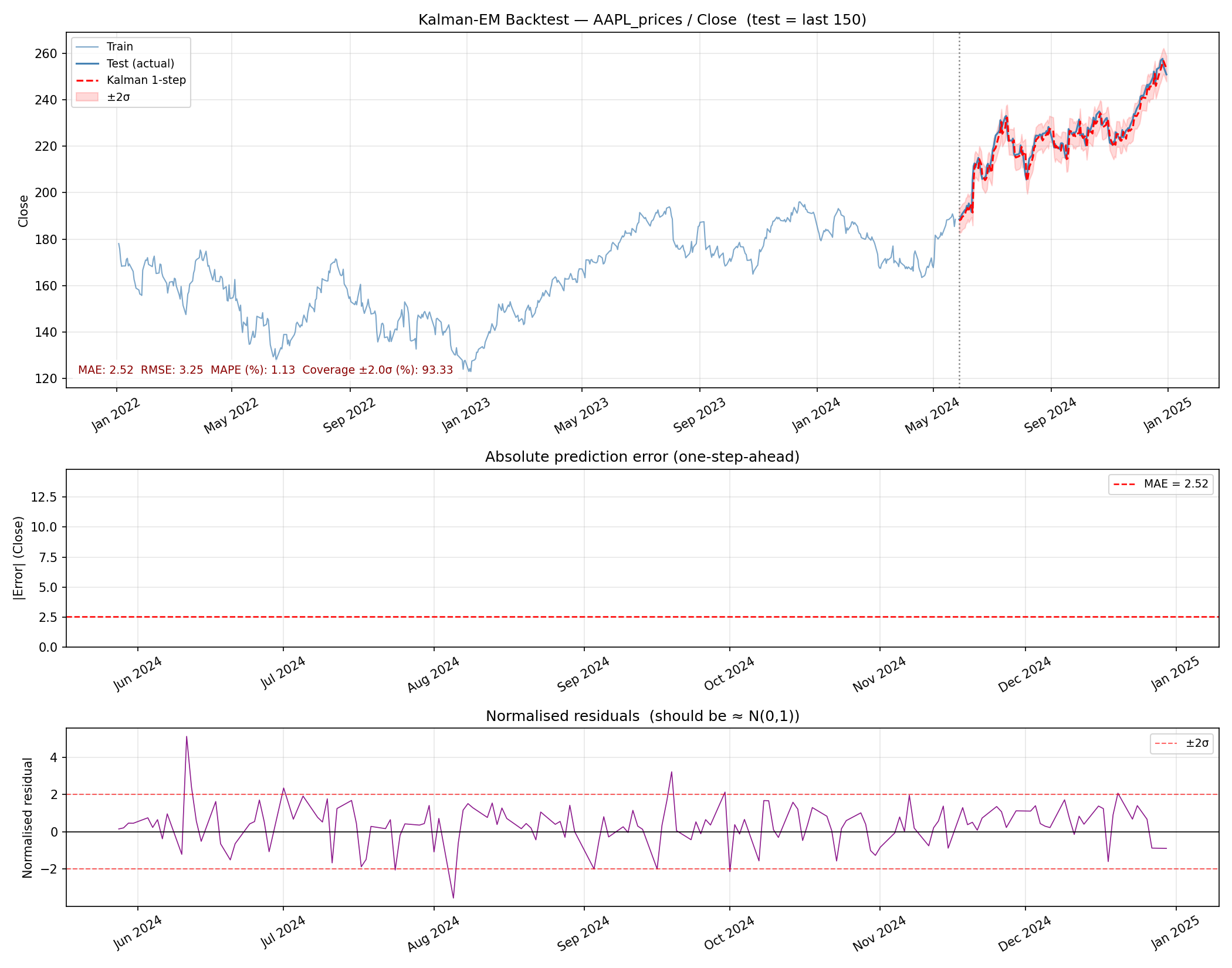
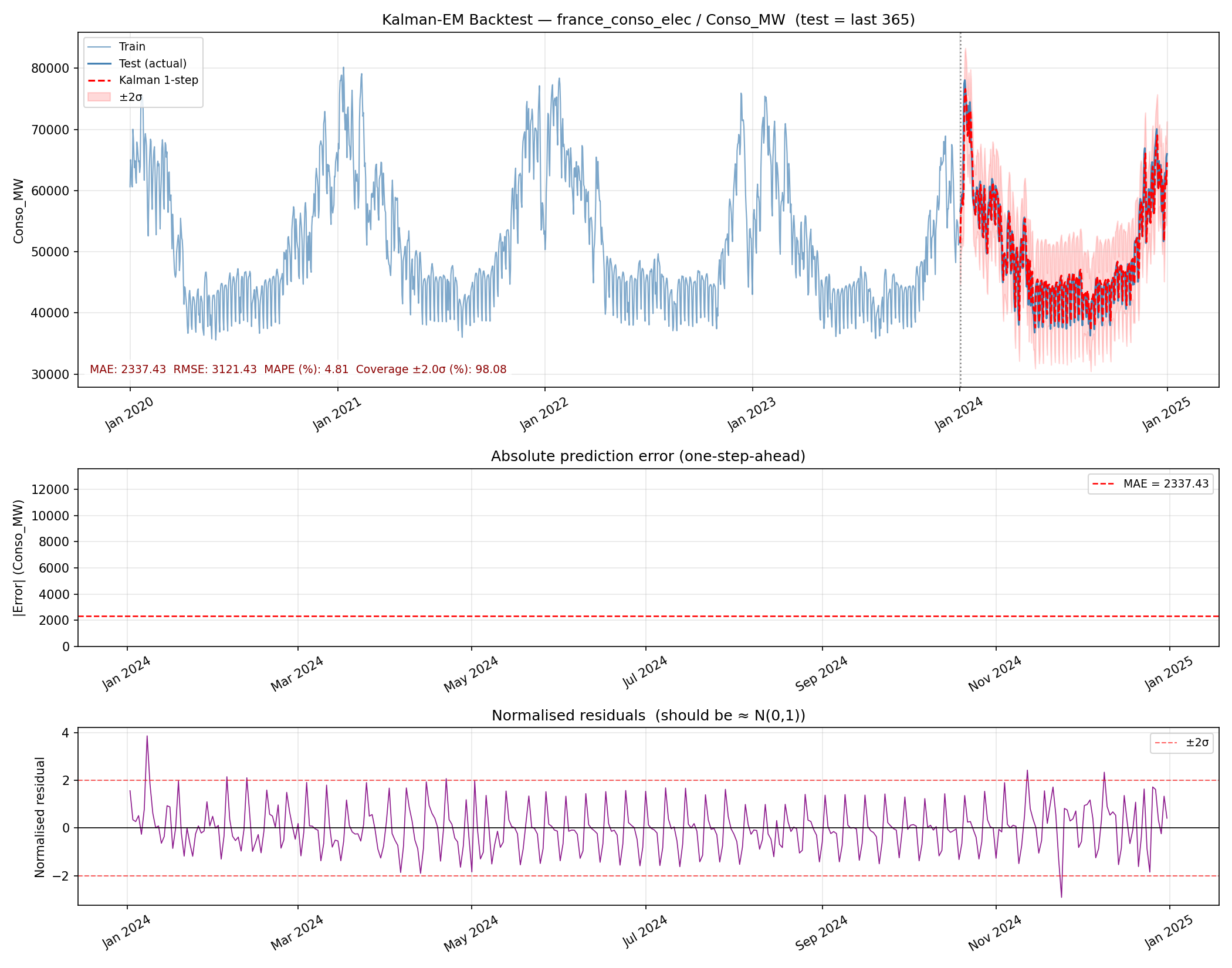
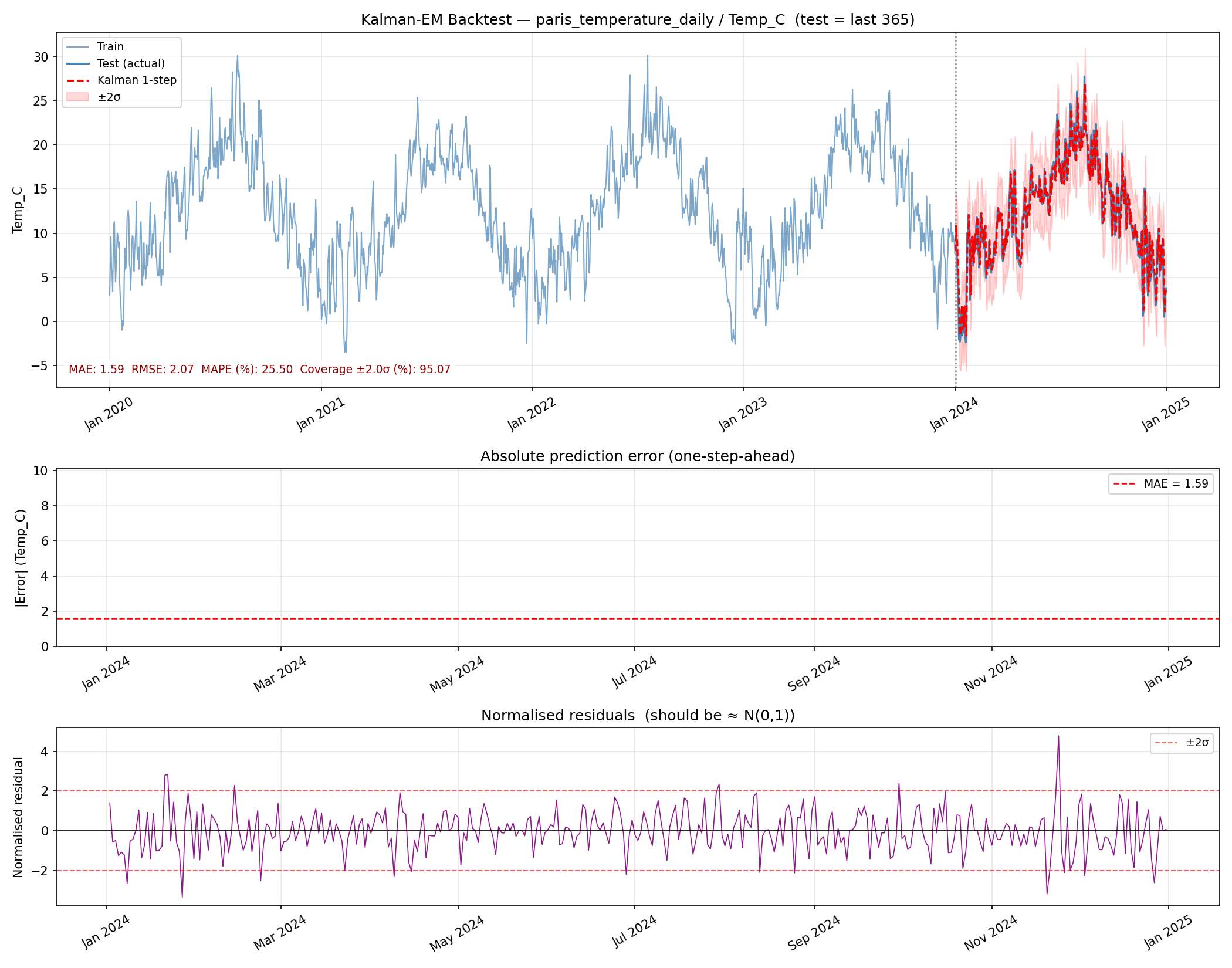
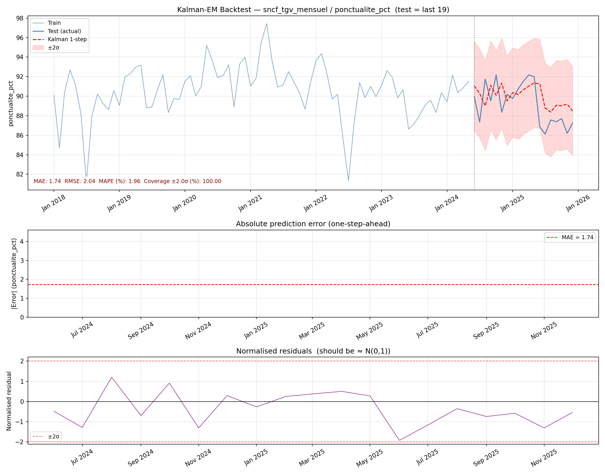
All results use one-step-ahead predictions on a held-out test set — the most honest evaluation strategy.
AAPL stock price — last 150 trading days
| MAE (USD) | RMSE (USD) | MAPE (%) | Coverage ±2σ (%) |
|---|---|---|---|
| 2.52 | 3.25 | 1.13 | 93.33 |
French electricity consumption — last 365 days
| MAE (MW) | RMSE (MW) | MAPE (%) | Coverage ±2σ (%) |
|---|---|---|---|
| 2 337 | 3 121 | 4.81 | 98.08 |
Paris daily temperature — last 365 days
| MAE (°C) | RMSE (°C) | Coverage ±2σ (%) |
|---|---|---|
| 1.59 | 2.07 | 95.07 |
MAPE is not reported: Celsius values near 0 °C in winter produce artifically high percentages.
SNCF TGV punctuality — last 19 months
| MAE (pp) | RMSE (pp) | MAPE (%) | Coverage ±2σ (%) |
|---|---|---|---|
| 1.74 | 2.04 | 1.96 | 100.00 |
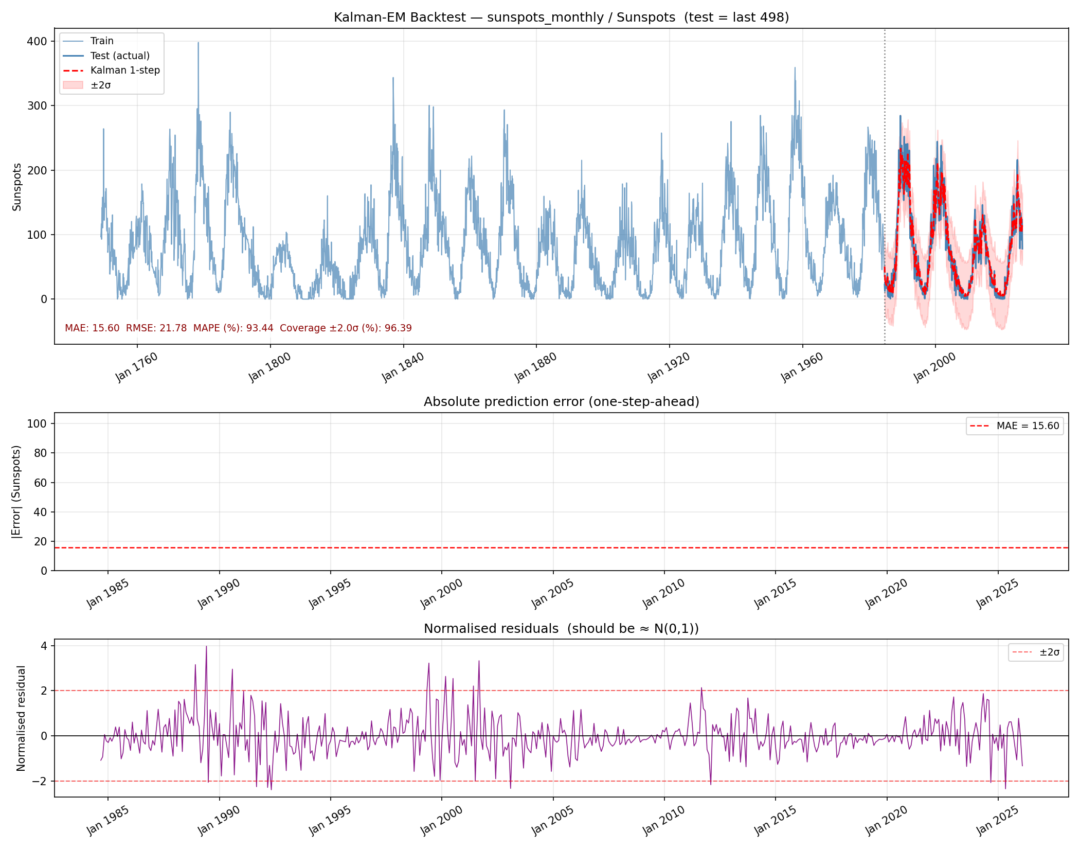
Monthly sunspot number — last 498 months (~41 years)
| MAE | RMSE | Coverage ±2σ (%) |
|---|---|---|
| 15.60 | 21.78 | 96.39 |
The ~11-year Schwabe cycle is quasi-periodic (period varies between 9 and 14 years) and non-stationary in amplitude — making this a genuinely challenging benchmark. MAPE is not reported because sunspot numbers regularly reach 0.
d=4captures the fundamental oscillation and its harmonics.
Documentation
| Document | Description |
|---|---|
docs/kalman_em_theory.pdf |
Full theoretical derivations: Kalman filter recursion, RTS smoother, EM E-step / M-step proofs, convergence theorem, prediction intervals |
docs/numerical_issues.md |
Numerical pitfalls encountered and fixes applied (Cholesky + solve, Joseph form, spectral clipping, STL pipeline) |
data/README.md |
Dataset provenance, column descriptions, API sources, licences |
Project structure
kalman_time_series/
│
├── app.py                        Streamlit Forecaster application
├── requirements.txt              Python dependencies
├── pyproject.toml                Package metadata (PyPI)
├── README.md                     This file
│
├── kalman_em/                    Core library
│   ├── __init__.py
│   ├── kalman_filter.py          Kalman filter + RTS smoother (Cholesky, Joseph form)
│   ├── em.py                     EM algorithm (E-step / M-step, n_restarts)
│   └── model.py                  KalmanEM public class
│
├── examples/                     Ready-to-run scripts
│   ├── evaluate.py               Generic one-step-ahead backtest (--col)
│   ├── stock_prediction.py       AAPL smoothing + forecast
│   ├── energy_prediction.py      French electricity (STL + Kalman-EM)
│   ├── transport_prediction.py   SNCF TGV traffic (STL + Kalman-EM)
│   └── sunspot_prediction.py     Solar cycle backtest
│
├── data/                         Local CSV datasets
│   ├── AAPL_prices.csv
│   ├── france_conso_elec.csv
│   ├── sncf_tgv_mensuel.csv
│   ├── paris_temperature_daily.csv
│   ├── sunspots_monthly.csv
│   └── README.md
│
├── assets/                       Backtest result figures (auto-generated)
│
├── tests/                        pytest test suite (39 tests)
│   ├── test_kalman_filter.py
│   ├── test_em.py
│   └── test_model.py
│
└── docs/                         Documentation
    ├── kalman_em_theory.pdf       Theoretical foundations
    └── numerical_issues.md        Numerical best practices
Licence
Data files are distributed under their original licences (see data/README.md).
Source code is provided for educational and research purposes.
Project details
Verified details
These details have been verified by PyPIProject links
GitHub Statistics
Maintainers


Download files
Download the file for your platform. If you're not sure which to choose, learn more about installing packages.
Source Distribution
Built Distribution
Filter files by name, interpreter, ABI, and platform.
If you're not sure about the file name format, learn more about wheel file names.
Copy a direct link to the current filters
File details
Details for the file kalman_em-0.2.2.tar.gz.
File metadata
- Download URL: kalman_em-0.2.2.tar.gz
- Upload date:
- Size: 23.7 kB
- Tags: Source
- Uploaded using Trusted Publishing? Yes
- Uploaded via: twine/6.1.0 CPython/3.13.7
File hashes
| Algorithm | Hash digest | |
|---|---|---|
| SHA256 |
ce44a1ffeb37f1e1664585a08347684c7fdd03ab5add7941986e850ce4be237f
|
|
| MD5 |
8c0996688e34862ab4919751e3adeab2
|
|
| BLAKE2b-256 |
1b5fdca8e41380c3685c5a4f7d489f73cbcbef080ebc111cc70f01b1ffeea197
|
Provenance
The following attestation bundles were made for kalman_em-0.2.2.tar.gz:
Publisher:
publish.yml on MarouaneAEF/kalman_time_series
-
Statement:
-
Statement type:
https://in-toto.io/Statement/v1 -
Predicate type:
https://docs.pypi.org/attestations/publish/v1 -
Subject name:
kalman_em-0.2.2.tar.gz -
Subject digest:
ce44a1ffeb37f1e1664585a08347684c7fdd03ab5add7941986e850ce4be237f - Sigstore transparency entry: 1026416029
- Sigstore integration time:
-
Permalink:
MarouaneAEF/kalman_time_series@18dd7f788cb106f867032a4bdcba695387015c4e -
Branch / Tag:
refs/tags/v0.2.2 - Owner: https://github.com/MarouaneAEF
-
Access:
public
-
Token Issuer:
https://token.actions.githubusercontent.com -
Runner Environment:
github-hosted -
Publication workflow:
publish.yml@18dd7f788cb106f867032a4bdcba695387015c4e -
Trigger Event:
push
-
Statement type:
File details
Details for the file kalman_em-0.2.2-py3-none-any.whl.
File metadata
- Download URL: kalman_em-0.2.2-py3-none-any.whl
- Upload date:
- Size: 15.5 kB
- Tags: Python 3
- Uploaded using Trusted Publishing? Yes
- Uploaded via: twine/6.1.0 CPython/3.13.7
File hashes
| Algorithm | Hash digest | |
|---|---|---|
| SHA256 |
acc330e14dcda15bb1b6871dccbfa16c5d33070658f5bef8f6f068bba921720a
|
|
| MD5 |
bf28d6f74616d0afeb294d12f5da57e1
|
|
| BLAKE2b-256 |
cedf289536d4e12f311fc801e6431c15a5c59006b046cccebfb1687cfdf1d8e3
|
Provenance
The following attestation bundles were made for kalman_em-0.2.2-py3-none-any.whl:
Publisher:
publish.yml on MarouaneAEF/kalman_time_series
-
Statement:
-
Statement type:
https://in-toto.io/Statement/v1 -
Predicate type:
https://docs.pypi.org/attestations/publish/v1 -
Subject name:
kalman_em-0.2.2-py3-none-any.whl -
Subject digest:
acc330e14dcda15bb1b6871dccbfa16c5d33070658f5bef8f6f068bba921720a - Sigstore transparency entry: 1026416077
- Sigstore integration time:
-
Permalink:
MarouaneAEF/kalman_time_series@18dd7f788cb106f867032a4bdcba695387015c4e -
Branch / Tag:
refs/tags/v0.2.2 - Owner: https://github.com/MarouaneAEF
-
Access:
public
-
Token Issuer:
https://token.actions.githubusercontent.com -
Runner Environment:
github-hosted -
Publication workflow:
publish.yml@18dd7f788cb106f867032a4bdcba695387015c4e -
Trigger Event:
push
-
Statement type:






