Spectral reduction and analysis package for the Kast optical spectrograph

Project description
kastredux
Specialized Lick/KAST optical spectral reduction package
Installation
kastredux can be installed from pip:
pip install kastredux
or from git:
git clone https://github.com/aburgasser/kastredux.git
cd kastredux
python -m setup.py install
It is recommended that you install in a conda environment to ensure the dependencies do not conflict with installations of other packages
conda create -n kastredux python=3.13
conda activate kastredux
kastredux uses the following external packages:
astropy: https://www.astropy.org/matplotlib: https://matplotlib.org/numpy<2.0: https://numpy.org/pandas: https://pandas.pydata.org/scipy: https://scipy.org/
Resources
kastredux comes equipped with several spectral files of use in calibration and analysis of low mass stellar data:
Flux standards
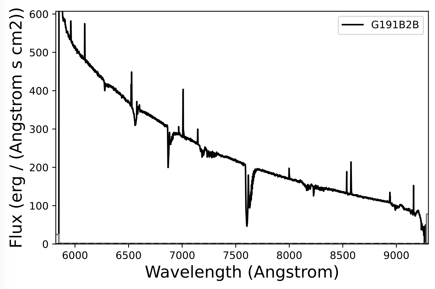
The code includes spectrophotometric flux standards from Oke (1990), Hamuy et al. (1992) , and Hamuy et al. (1994); see ESO's pages on Oke standards and Hamuy standards.
Spectral standards
- SDSS K and M dwarf. subdwarf, and giant spectral templates from Kesseli et al. (2017) and Kesseli et al. (2019).
- SDSS M and L dwarf spectral templates from Bochanski et al. (2007) and Schmidt et al. (2014).
- Low metallicity M subdwarf optical standards from Lepine et al. (2007).
- L dwarf optical standards from Kirkpatrick et al. (1999).
- T dwarf optical standards from Burgasser et al. (2003).
Telluric standards
OBAFGKM standards from the Pickles (1998) library.
Sample spectra
The code also includes reduced spectra from Kast for the following sources in *.fits format:
- G 233-42: M5 dwarf, G=14.0
- PM J0102+5254: M3 dwarf, G=12.5
- LP 555-25: M6.5 dwarf, G=15.8
- TOI-2084: M2 dwarf, G=14.4, data from Barkaoui et al. (2003)
- LP 389-13: M2 dwarf, G=11.6, data from Rothermich et al. (2024)
Reduction
kastredux includes a semi-automated pipeline for reducing optical spectra with the Kast RED and BLUE cameras for these dispersers (those in bold are fully tested)
- RED: 300/4230, 300/7500, 600/3000, 600/5000, 600/7500, 830/8460, 1200/5000
- BLUE: 452/3306, 600/4310, 830/3460
- LDSS-3: VPH-RED (experimental)
The main steps conducted by the reduction programs include:
- Creation of reduction script from fits files
- Creation of bias, flat field, and masking arrays
- Calibration of science images
- Determination of wavelength solution from arc lamps
- Spectral dispersion tracing using bright stars
- Boxcar and optimal extraction of 1D spectrum with background subtraction
- Flux calibration with spectrophotometric standard
- Telluric correction and secondary flux calibration with G2 or A0 flux standard
These steps are conducted using the following calls:
Generate instructions
The first step for reduction is to use the acquired data to generate an instruction file, and to edit the file to ensure sources are assigned correctly. Assuming all of the data are contained in a folder data:
import kastredux as kr
kr.makeInstructions("data",savelog=True)
This will create a reductions folder parallel to data generate two instruction files: input.txt and input_blue.txt, which include lines indicating the relevant files for flats, biases, and arcs; and tab-delimited lines providing extraction information for the flux calibrator (FLUXCAL), telluric stars (TELLURIC) and science targets (SOURCE). Baseline parameters are preset, and these can be modified or additional source extractions added as needed.
The keyword savelog=True also generates the CSV files log_[date]_RED.csv and log_[date]_BLUE.csv generated from the fits files which includes guesses on what sources are arcs, flats, biases, science, telluric standard, and flux calibrators.
At this stage, it is helpful to review the instruction files and make edits, including:
- File numbers (
FILES=###-###), useful if there were initial "test" exposures - Source names (
NAME=) - Flux calibrator (
FLUXCAL) - note that at least one catalogued flux calibrator must be included - Initial guess for the center of the spectral trace (
CENTER=###) - Extraction window around center trace (
WINDOW=###) - Regions around center trace to sample the background (
BACK=NNN,MMM) - Telluric star assignment (
TELLURIC=)
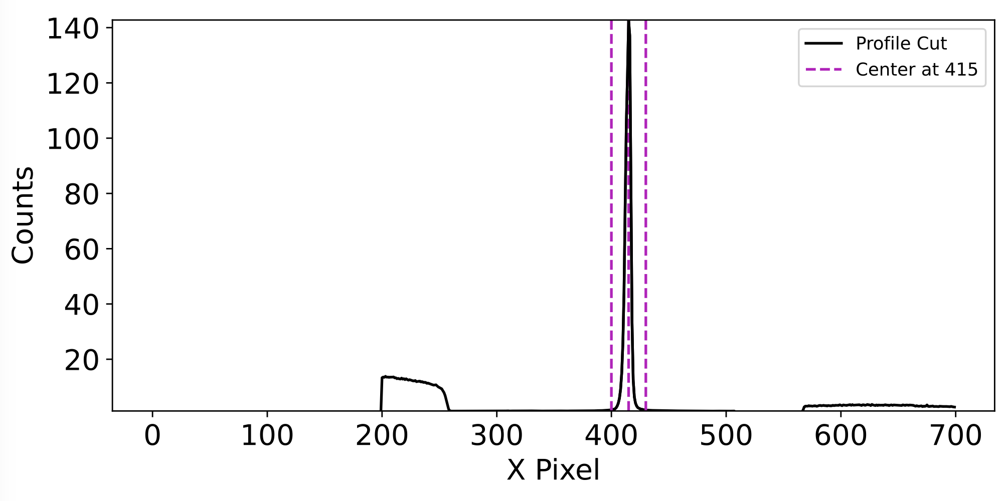
You can check the initial centering of spectral traces by inspecting spatial profiles:
kr.profileCheck("data/input.txt",verbose=True)
In addition to listing the source extraction centers (verbose=True), this function will produce a series of PDF files diagnostic_profile_[NAME]_[RED/BLUE].pdf which can be used to inspect spatial source centering.
Finally, there are additional keywords that can be added to the SOURCE lines to help with extraction:
RECENTER= True (default): set to False to use the initial center guess as a fixed number, useful for faint sources or source in close proximity to each otherAPPLY_TRACE= False (default): set to True to use the profile trace from the Telluric standard, useful for faint sources or source in close proximity to each other
Run bulk extraction code
When you are happy with the instruction file, the full reduction can be called with the command:
kr.reduce(instructions="data/input.txt",reset=True,verbose=True)
The keywords reset=True means it will overwrite prior extractions, while verbose=True gives detailed feedback in the output.
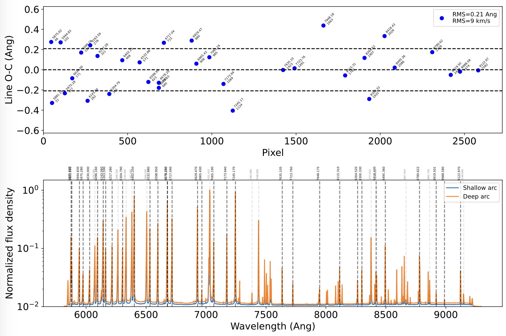
Assuming everything goes well, the following diagnostic plots will be generated to check the reductions:
diagnostic_wavecal_[NAME]_[RED/BLUE].pdf: two-panel plot showing the difference between arc line location and wavelength calibration fit (including RMS in Angstroms and km/s), and the arc spectrum as a function of wavelength with fit lines labeled.
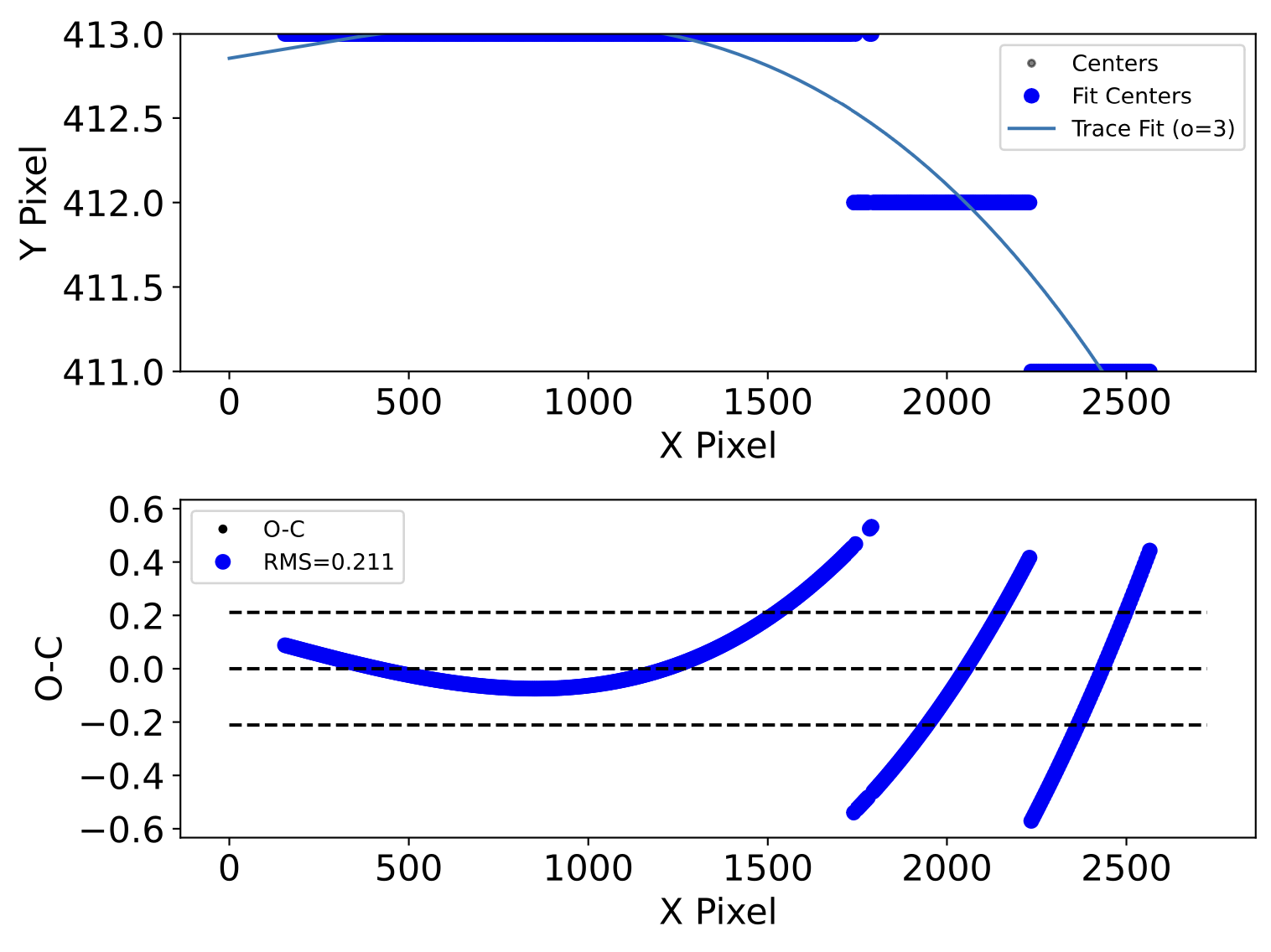
diagnostic_trace_[NAME]_[RED/BLUE].pdf: two-panel plot showing the trace (peak count pixel) as a function of X and Y pixel coordinate and the trace fit, and difference between peak pixels and trace fit
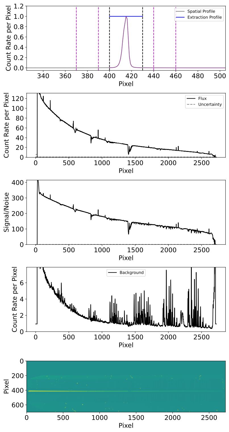
diagnostic_extraction_[NAME]_[RED/BLUE].pdf: five-panel plot showing the spatial profile, extracted count rate, signal-to-noise, background count rate, and 2D image around source trace
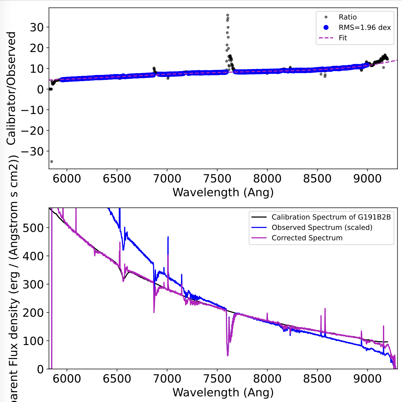
diagnostic_fluxcal_[RED/BLUE].pdf: two-panel plot showing the ratio of calibrated to observed count rate for the flux calibrator and correction fit, and comparing the calibrated, observed, and corrected flux calibrator spectra
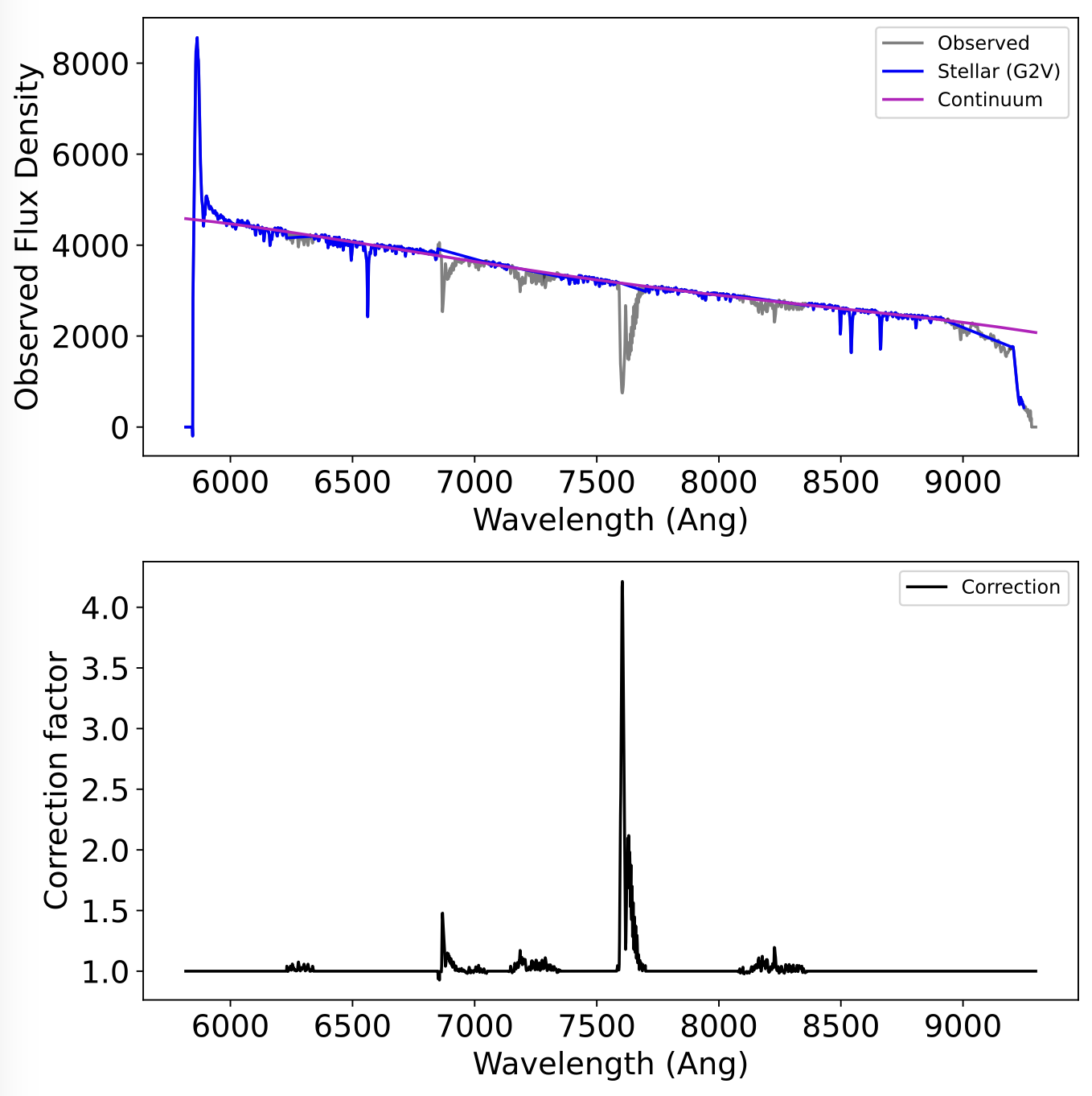
diagnostic_telluric_[NAME]_[RED/BLUE].pdf: two-panel plot illustrating the observed telluric spectrum with telluric regions masked, and the telluric correction spectrum.
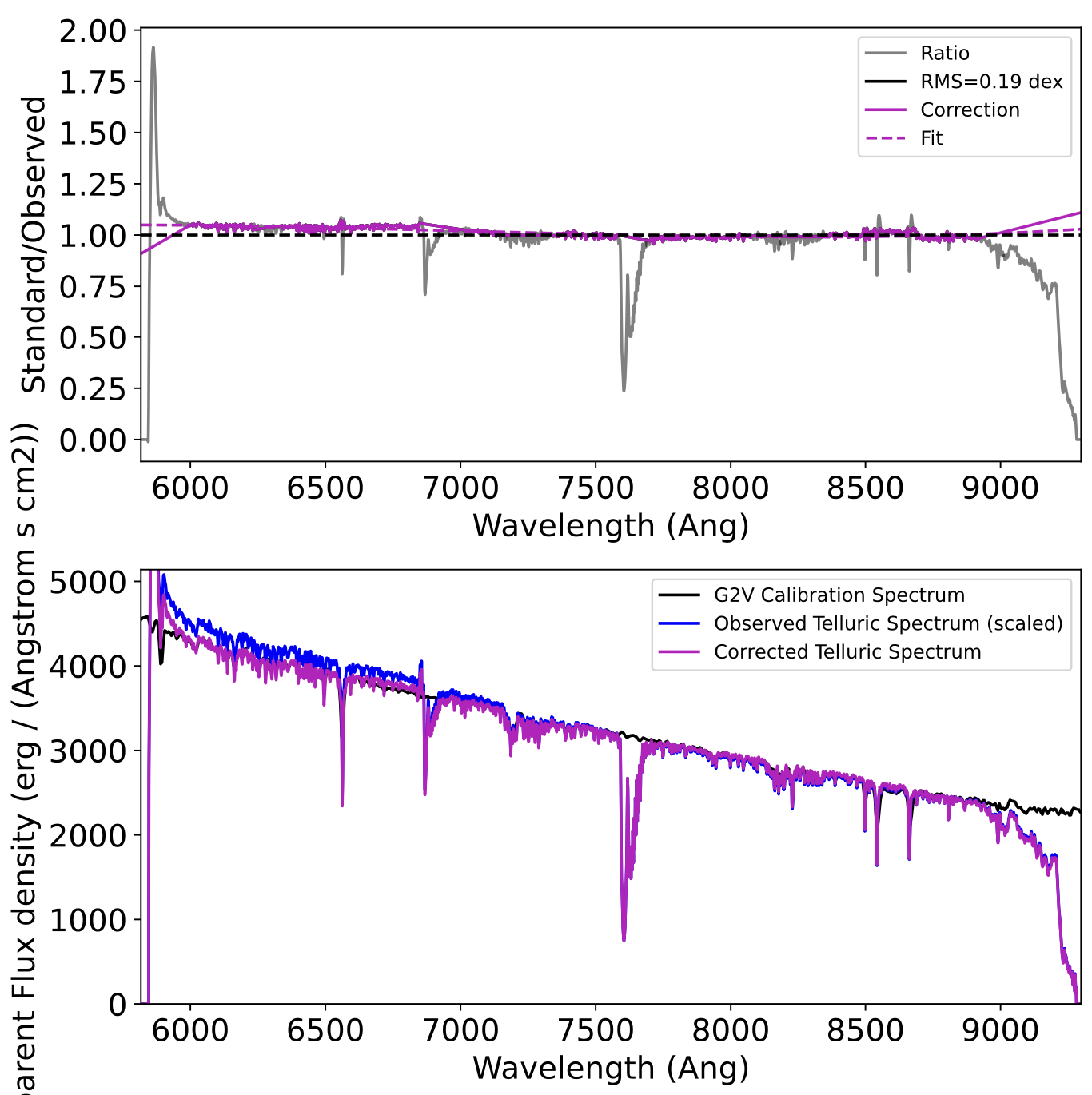
diagnostic_reflux_[NAME]_[RED/BLUE].pdf: two-panel plot showing the ratio of observed and model telluric spectrum and corresponding correction function, and comparing the model, observed, and corrected telluric spectra
kast[RED/BLUE]_[NAME]_[DATE].pdf: Final spectrum
It is recommended to evaluate the diagnostic plots and adjust the instruction files as needed.
The output fits file include:
bias_[RED/BLUE].fits: bias fileflat_[RED/BLUE].fits: normalized flatfield filemask_[RED/BLUE].fits: mask filekast[RED/BLUE]_[NAME]_[DATE].fits: Final spectrum
There are also a series of pickle (*.pkl) files containing intermediate data products.
Extraction step-by-step
It is also possible to conduct reductions step-by-step if more control over the process is desired with the following steps:
- Set up necessary information
Start with import statements and the variables needed for your reduction; the *f variables correspond to image frame numbers
import kastredux as kr
import numpy as np
import os

data_folder = "data"
reduction_folder = "reduction"
camera = "RED"
grating = "600/7500"
prefix = "r"
darkf1,darkf2 = 1000,1010
baisf1,biasf2 = 1000,1010
arcf = 1021
scif1,scif2 = 1030,1031
sciname = "RedStar"
flxf = 1030
flxname = "Hiltner600"
tellf = 1040
- Generate calilbration frames
First make the bias frame
files = ["{}{}.fits".format(prefix,int(n)) for n in np.arange(darkf1,darkf2)]
bias_out = os.path.join(reduction_folder,"bias{}.fits",format(camera))
bias, _ = kr.makeBias(files,folder=data_folder,mode=camera,output=bias_out)
Then make the normalized flat field frame
files = ["{}{}.fits".format(prefix,int(n)) for n in np.arange(baisf1,biasf2)]
flat_out = os.path.join(reduction_folder,"flat{}.fits",format(camera))
flat, _ = kr.makeBias(files,bias,folder=data_folder,mode=camera,output=flat_out)
Then make the mask frame from the bias and flatfield
mask_out = os.path.join(reduction_folder,"mask{}.fits",format(camera))
mask = kr.makeMask(bias,flat,mode=camera,output=mask_file)
flatc = kr.maskClean(flat,mask,replace=1.)
Finally generate the wavelength calibration
arc,_ = kr.readFiles("{}{}.fits".format(prefix,int(arcf)),folder=data_folder,mode=camera)
diagplot = "diagnostic_wavecal.pdf"
wavecal = kr.waveCalibrateArcs(arc,,dispersion=grating,mode=camera,middle=True,plot_file=diagplot)
- Generate flux calibration
Use your flux calibrator observation to make the flux correction function
im,hd = kr.readFiles("{}{}.fits".format(prefix,int(flxf)),folder=data_folder,mode=camera)
imr,var = kr.reduceScienceImage(im,bias,flat,mask,hd=hd)
cntr = kr.findPeak(imr)
trace = kr.traceDispersion(imr,cntr=cntr,window=10,method='maximum')
imrect = kr.rectify(imr,trace)
varrect = kr.rectify(var,trace)
maskrect = kr.rectify(mask,trace)
flatrect = kr.rectify(flat,trace)
arcrect = kr.rectify(arc,trace)
cntr = kr.findPeak(imrect,cntr=cntr,window=10)
diagplot = "diagnostic_extraction_fluxstd.pdf"
flxsp = kr. extractSpectrum(imrect,cntr=cntr,var=varrect,mask=maskrect,src_wnd=10,bck_wnd="20,40",method="boxcar",plot_file=diagplot)
wavecal_new = kr.waveCalibrateArcs(arcrect,cntr=cntr,prior=wavecal,mode=camera)
flxsp.applyWaveCal(wavecal_new)
diagplot = "diagnostic_fluxcal.pdf"
fluxcal = kr.fluxCalibrate(flxsp,flxname,fit_order=fit_order,fit_scale=flux_fit_scale,fit_range=[6000,9000],plot_file=diagplot
- Generate telluric correction
Use your G2V telluric star (if obtained) to make the second-order flux correction and telluric correction functions
im,hd = kr.readFiles("{}{}.fits".format(prefix,int(tellf)),folder=data_folder,mode=camera)
imr,var = kr.reduceScienceImage(im,bias,flat,mask,hd=hd)
cntr = kr.findPeak(imr)
trace = kr.traceDispersion(imr,cntr=cntr,window=10,method='maximum')
imrect = kr.rectify(imr,trace)
varrect = kr.rectify(var,trace)
maskrect = kr.rectify(mask,trace)
flatrect = kr.rectify(flat,trace)
arcrect = kr.rectify(arc,trace)
cntr = kr.findPeak(imrect,cntr=cntr,window=10)
diagplot = "diagnostic_extraction_tellstd.pdf"
tellsp = kr. extractSpectrum(imrect,cntr=cntr,var=varrect,mask=maskrect,src_wnd=10,bck_wnd="20,40",method="boxcar",plot_file=diagplot)
wavecal_new = kr.waveCalibrateArcs(arcrect,cntr=cntr,prior=wavecal,mode=camera)
tellsp.applyWaveCal(wavecal_new)
tellsp.applyFluxCal(fluxcal)
diagplot = "diagnostic_telluric.pdf"
tellcorr = kr.telluricCalibrate(tellsp,spt="G2V",plot_file=diagplot)
diagplot = "diagnostic_reflux_tellstd.pdf"
tellfluxcorr = kr.fluxReCalibrate(tellsp,spt="G2V",plot_file=diagplot)
- Extract science spectrum
This case uses the trace from the telluric standard, and applies flux calibration and telluric correction
files = ["{}{}.fits".format(prefix,int(n)) for n in np.arange(scif1,scif2)]
ims,_ = kr.readFiles(files,folder=data_folder,mode=camera)
im = crRejectCombine(ims,verbose=verbose)
imr,var = kr.reduceScienceImage(im,bias,flat,mask,hd=flxhd)
imrect = kr.rectify(imr,trace)
varrect = kr.rectify(var,trace)
maskrect = kr.rectify(mask,trace)
flatrect = kr.rectify(flat,trace)
arcrect = kr.rectify(arc,trace)
cntr = kr.findPeak(imrect,cntr=cntr,window=10)
diagplot = "diagnostic_extraction_science.pdf"
scisp = kr. extractSpectrum(imrect,cntr=cntr,var=varrect,mask=maskrect,src_wnd=10,bck_wnd="20,40",method="boxcar",plot_file=diagplot)
wavecal_new = kr.waveCalibrateArcs(arcrect,cntr=cntr,prior=wavecal,mode=camera)
scisp.applyWaveCal(wavecal_new)
scisp.applyFluxCal(fluxcal)
scisp.applyFluxCal(tellfluxcorr)
scisp.applyTelluricCal(tellcorr)
Analysis
kastredux comes with several routines for analyzing optical spectra of low-mass stars and brown dwarfs. These routines operate on an Spectrum class object that contains the spectral data and allows for various spectral operations.
Spectrum class
The kastredux Spectrum class is the primary data object for spectral data, and is similar to the astropy specutils class. In addition to arrays for wavelength, flux, uncertainty, variance and masking, the internal functions for the Spectrum class include:
- spectral math: built in functions are provided to add, subtract, multiple, and divide spectra, accounting for the appropriate wavelength solution and uncertainty propagation
scale(val): scale the flux and variance by a constant valuesample([w1,w2],method="median"): sample the spectrum in a specified wavelength range using the specified statisticnormalize([w1,w2]): scale the spectrum based on the maximum flux in a specified wavelength rangetrim([w1,w2]): trim the spectrum to the specified wavelength rangeshift(val): shift the spectrum by a constant wavelength or velocitysmooth(width): apply a smoothing profile of a given pixel widthcleanCR(): cleans discrepant pixels in the spectrumapplyMask(mask): applies a pixel mask, where the mask array specifies pixels to exclude as either True or 1maskWave([w1,w2]): mask pixels in a specified wavelength rangeapplyWaveCal(wavecal): applies the wavelength calibration computed inkr.waveCalibrateArcs()applyFluxCal(fluxcal): applies the flux calibration computed inkr.fluxCalibrate()applyTelluricCal(tellcal): applies the telluric correction computed inkr.telluricCalibrate()redden(val): applies a reddening to a spectrum using the Cardelli, Clayton, and Mathis (1989) modelreset(): reset the Spectrum object to its original read in stateconvertWave(unit): convert wavelength array to the given wavelength unitconvertFlux(unit): convert flux and uncertainty arrays to the given flux unitplot(): plots the spectrum for visualizationtoFile(file): saves the spectrum to a file, including fits and tab-delimited ascii files
Spectrum class objects can be initiated through a file name or specifying wavelength, flux, and uncertainty arrays:
import kastredux as kr
sp = kr.Spectrum('kast_spectrum.fits")

import astropy.unit as u
wave_unit = u.Angstrom # default
flux_unit = u.erg/u.s/u.cm/u.cm/u.Angstrom # default
sp = kr.Spectrum(wave=[array]*wave_unit,flux=[array]*flux_unit,unc=[array]*flux_unit),
Analysis routines
The `kastredux' analysis routines are defined primarily for late-type stars and brown dwarfs (M, L, and T dwarfs). These are the functions currently defined that operate on the Spectrum class objects (sp):
compareSpectra(sp1,sp2): compares two spectra using a defined statisticclassifyTemplate(sp): compares a spectrum to defined templates initiated usinginitializeStandards()measureIndex(sp,ranges,sample="median",method="ratio"): measures a spectral index defined by wavelengths specified in the ranges array, where sample describes how the spectral flux is measured and method describes how the fluxes are combinedmeasureIndexSet(sp,ref="lepine2003): measures a predefined set of spectral indices; call asmeasureIndexSet(info=True)to obtain a current list of spectral indicesclassifyIndices(sp,ref="lepine2003): computes a spectral type from a predefined set of spectral indices; call asclassifyIndices(info=True)to obtain a current list of spectral indicesmeasureEW(sp,w0): computes the equivalent width of a feature centered at wavelength w0measureEWElement(sp,element): computes the equivalent widths for transitions of a given elementmeasureEWSet(sp,ref='mann2013'): computes the equivalent widths for a predefined set of linesmetallicity(sp,ref='mann2013'): determines the metallicity from an empirical calibration of the zeta indexchiFactor(sp,ref='schmidt2014'): computes the chi correction factor, and if desired the relative Halpha to bolometric luminosity using a predefined spectral-type based calibration
The function kr.theWorks(sp) runs all of these analysis routines together
Citing the code
If you use this code in your research, publications, or presentations, please include the following citation:
Burgasser (2026). aburgasser/kastredux (vXXX). Zenodo. https://doi.org/10.5281/zenodo.18333308
or in bibtex:
@software{adam_burgasser_2026_18333308,
  author       = {Adam Burgasser},
  title        = {aburgasser/kastredux: vXXX},
  month        = jan,
  year         = 2026,
  publisher    = {Zenodo},
  version      = {v1.1},
  doi          = {10.5281/zenodo.18333308},
  url          = {https://doi.org/10.5281/zenodo.18333308},
}
where (vXXX) corresponds to the version used.


Download files
Download the file for your platform. If you're not sure which to choose, learn more about installing packages.
Source Distribution
Built Distribution
Filter files by name, interpreter, ABI, and platform.
If you're not sure about the file name format, learn more about wheel file names.
Copy a direct link to the current filters
File details
Details for the file kastredux-1.1.3.tar.gz.
File metadata
- Download URL: kastredux-1.1.3.tar.gz
- Upload date:
- Size: 90.4 MB
- Tags: Source
- Uploaded using Trusted Publishing? Yes
- Uploaded via: twine/6.1.0 CPython/3.13.7
File hashes
| Algorithm | Hash digest | |
|---|---|---|
| SHA256 |
a5151365c192ca3a9474b6689aecb24e1ed0f841547409a8e59b5fee982b4f8a
|
|
| MD5 |
f79235c9c8f3f58c54fc32f775f0027b
|
|
| BLAKE2b-256 |
1e5a1b99fe4f3f9c7d11d0f147f6a8edf0d012cce0ad0358ee44473cbecc0025
|
Provenance
The following attestation bundles were made for kastredux-1.1.3.tar.gz:
Publisher:
python-publish.yml on aburgasser/kastredux
-
Statement:
-
Statement type:
https://in-toto.io/Statement/v1 -
Predicate type:
https://docs.pypi.org/attestations/publish/v1 -
Subject name:
kastredux-1.1.3.tar.gz -
Subject digest:
a5151365c192ca3a9474b6689aecb24e1ed0f841547409a8e59b5fee982b4f8a - Sigstore transparency entry: 929618525
- Sigstore integration time:
-
Permalink:
aburgasser/kastredux@3cbe200b0ab3412ead4a698a1a93668fd06c87df -
Branch / Tag:
refs/tags/v1.1.3 - Owner: https://github.com/aburgasser
-
Access:
public
-
Token Issuer:
https://token.actions.githubusercontent.com -
Runner Environment:
github-hosted -
Publication workflow:
python-publish.yml@3cbe200b0ab3412ead4a698a1a93668fd06c87df -
Trigger Event:
release
-
Statement type:
File details
Details for the file kastredux-1.1.3-py3-none-any.whl.
File metadata
- Download URL: kastredux-1.1.3-py3-none-any.whl
- Upload date:
- Size: 90.4 MB
- Tags: Python 3
- Uploaded using Trusted Publishing? Yes
- Uploaded via: twine/6.1.0 CPython/3.13.7
File hashes
| Algorithm | Hash digest | |
|---|---|---|
| SHA256 |
5366ef63114361672fe34ba0aa6151ca62cf62607cfd3726c9dd41907f1d14cf
|
|
| MD5 |
cd63de42417a45dfca552aeeba00dcec
|
|
| BLAKE2b-256 |
9bea6fb3433ea9db0489ad4c117603473d6adfea72f3673ad70173bdb7586c0c
|
Provenance
The following attestation bundles were made for kastredux-1.1.3-py3-none-any.whl:
Publisher:
python-publish.yml on aburgasser/kastredux
-
Statement:
-
Statement type:
https://in-toto.io/Statement/v1 -
Predicate type:
https://docs.pypi.org/attestations/publish/v1 -
Subject name:
kastredux-1.1.3-py3-none-any.whl -
Subject digest:
5366ef63114361672fe34ba0aa6151ca62cf62607cfd3726c9dd41907f1d14cf - Sigstore transparency entry: 929618526
- Sigstore integration time:
-
Permalink:
aburgasser/kastredux@3cbe200b0ab3412ead4a698a1a93668fd06c87df -
Branch / Tag:
refs/tags/v1.1.3 - Owner: https://github.com/aburgasser
-
Access:
public
-
Token Issuer:
https://token.actions.githubusercontent.com -
Runner Environment:
github-hosted -
Publication workflow:
python-publish.yml@3cbe200b0ab3412ead4a698a1a93668fd06c87df -
Trigger Event:
release
-
Statement type:


