Regime diagnostics for spatiotemporal kernels K(r,t) from non-equilibrium many-body systems

Project description
Kernel Dynamics Viewer (v0.8)
A small Python toolkit for regime diagnostics of spatiotemporal kernels
K(r, t) from non-equilibrium many-body systems (quantum or classical).
You measured or simulated a dynamic correlation function
K(r, t) = <O(r, t) O(0, 0)> — a spreading profile over space and time.
This tool turns it into a small set of measurable shape features and a
two-axis regime classification, with publication-style plots, in one
command:
kernel-viewer analyze data.npz
No theory, no interpretation — only numerical shape descriptors.
What it computes
| feature | definition | meaning |
|---|---|---|
transport exponent p |
late-window slope of log sigma^2(t) vs log t, boundary-contaminated tail excluded |
1 = diffusive, 2 = ballistic |
| unimodality score | 1 / n_peaks of the symmetrized profile (prominence-filtered) |
1.0 = single peak |
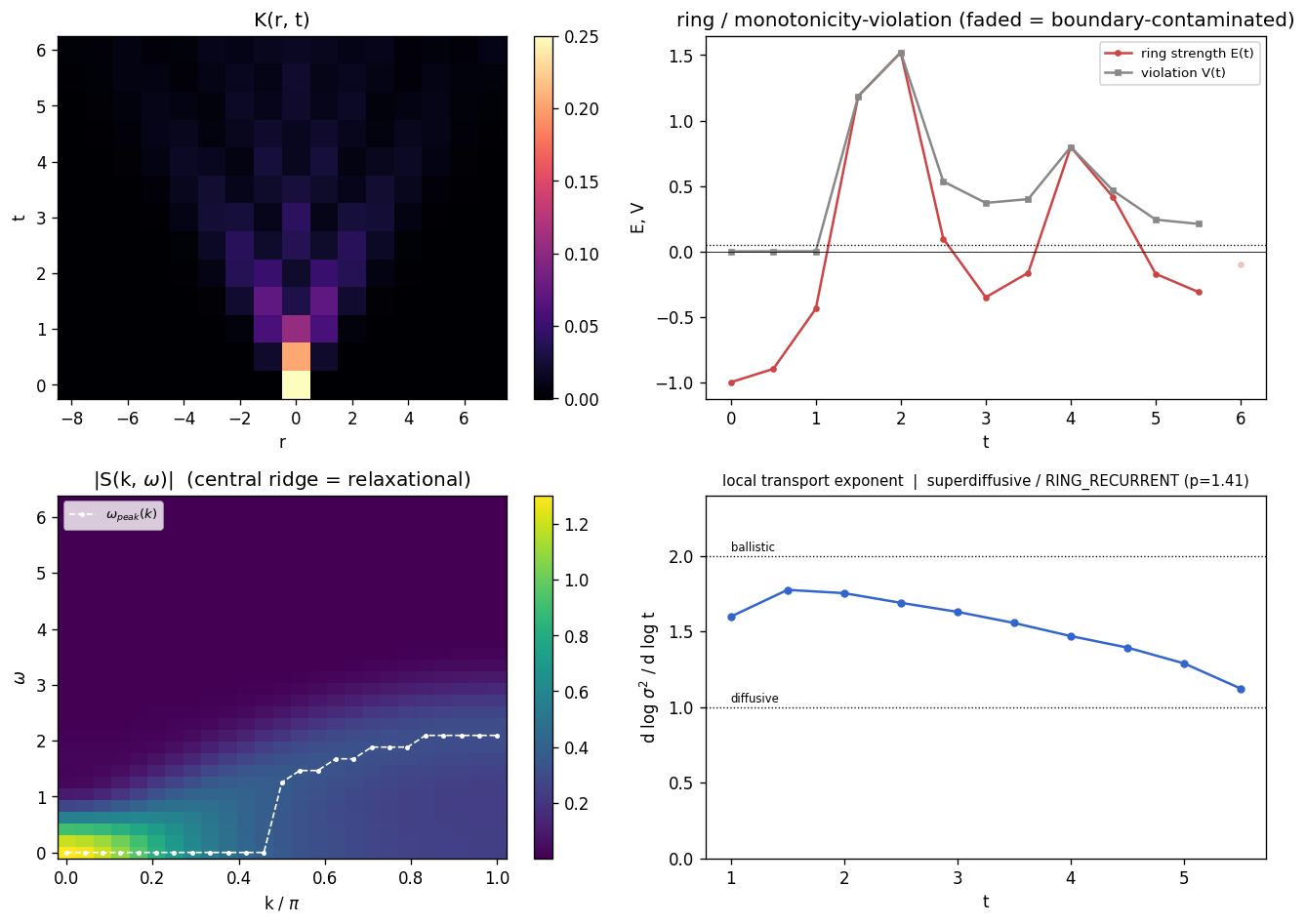
ring strength E(t) |
(max_{r>0} K - K(0)) / K(0) |
> 0: the maximum sits off the source |
violation V(t) |
strongest positive step of the profile, relative to K(0) |
0 = monotone profile |
| tail shape | gaussian / exponential / power-law, decided on the outer half of the profile via log-log curvature | power-law = heavy (Levy-like) tail |
S(k, omega) |
double cosine transform (Hann window) | central ridge = relaxational, off-axis ridge = propagating |
Two-axis classification
Axis 1 — transport (from the exponent + tail):
DIFFUSIVE / SUPERDIFFUSIVE / BALLISTIC / SUBDIFFUSIVE / LEVY
Axis 2 — coherence (from the ring history E(t)):
MONOTONE / RING_TRANSIENT / RING_PERSISTENT / RING_RECURRENT
The axes are deliberately independent, because they are in the data:
ballistic kernels can be unimodal, and diffusive systems can show transient
rings. "Chaotic vs integrable" is typically an axis-2 distinction
(transient vs recurrent rings), not an axis-1 one — that is why there is no
CHAOTIC transport class.
Two failure modes this design avoids:
unimodality ~ 1does not imply diffusive (early ballistic kernels are unimodal too) — transport is read fromsigma^2(t), never from peak counts;sigma^2 ~ tdoes not rule out Levy (for power-law tails the second moment is dominated by the finite window) — heavy tails are detected separately and promote the regime toLEVY.
Quickstart
pip install numpy scipy matplotlib
python -m kernel_viewer.cli demo            # 4 synthetic kernels -> reports + dashboards
python -m kernel_viewer.cli analyze examples/xxz_Sx_integrable.npz
python -m kernel_viewer.cli classify examples/ising_q_chaotic.npz -o report.json
Data format: .npz with K plus optional axes — 1D: K (T, R) with
r (R,), t (T,); 2D: K (T, Y, X) with x (X,), y (Y,), t (T,);
3D: K (T, Z, Y, X) with x, y, z, t; 4D: K (T, W, Z, Y, X)
with x, y, z, w, t. The time axis is always first. (Bare .npy works too; integer axes are then assumed.) The loader
dispatches on dimensionality automatically — no --dim flag is needed.
from kernel_viewer import load_kernel, classify
rep = classify(load_kernel("data.npz"))
print(rep.summary())
Input formats (v0.8)
load_any reads four formats and returns the same Kernel* objects regardless
of source, so the CLI accepts any of them (kernel-viewer classify data.mat):
| format | reader | notes |
|---|---|---|
.npz / .npy |
numpy |
the native format (above); load_any delegates to load_kernel unchanged |
.mat |
scipy.io.loadmat |
reads K (or the highest-dimensional non-private array) plus optional t and r/x/y/z/w. MATLAB is column-major and often stores time last ((R, T), (X, Y, T)); the time axis is detected from the coordinate lengths and moved to axis 0. Pass time_axis='first' or 'last' when the autodetect is ambiguous (it warns). |
.csv / .txt |
numpy.genfromtxt |
1D kernels only. layout='matrix' — a (T, R) grid; a NaN top-left corner marks a labelled grid with r along the first row and t down the first column. layout='long' — three columns t, r, K. Multi-dimensional kernels can't live unambiguously in a flat CSV and raise NotImplementedError; use .npz/.mat. |
from kernel_viewer import load_any, classify_any
rep = classify_any(load_any("data.mat", time_axis="last"))
print(rep.summary())
GUI (v0.8)
A Streamlit app turns the whole pipeline into a drag-and-drop dashboard:
pip install -e ".[gui]"             # Streamlit is an optional extra
streamlit run app/streamlit_app.py
Drop in a kernel (npz/npy/mat/csv) and the app runs the full analysis: the
regime summary (the exact classify_any text), the dimension-appropriate
matplotlib dashboard, and the stateflow axis timelines (continuous
transport slope and coherence E(t)) with the detected transitions. The
sidebar exposes the two real knobs — ring_threshold and edge_limit — at
their library defaults; nothing is auto-tuned. The core install stays
numpy + scipy + matplotlib; Streamlit is never imported by the library or the
core test suite.
| regime dashboard | stateflow axes |
|---|---|
 |
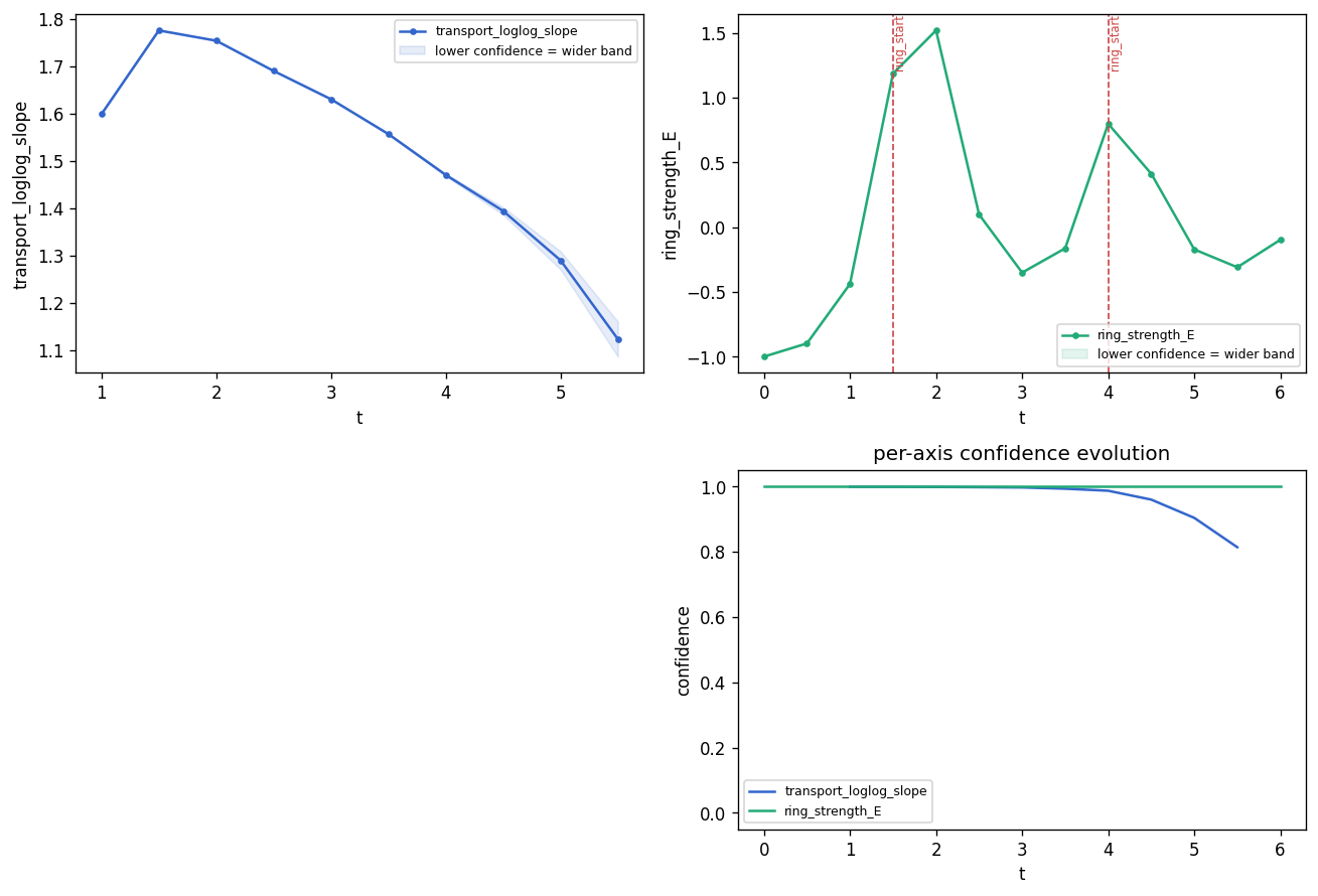 |
Planned (not in v0.8): Plotly interactivity, a K(r, t) time-slider
animation, and multi-file comparison — see app/README.md.
Deploy (Streamlit Community Cloud)
Live app: https://kernel-dynamics-viewer-mtrq39zmjxblbfptzs6evm.streamlit.app/
The app deploys on Streamlit Community Cloud with
no extra setup: point a new app at app/streamlit_app.py on the main
branch. Dependencies install from the repo-root requirements.txt (the
package + its gui extra; runtime.txt pins Python 3.12). The app resolves the
bundled examples/*.npz from its own file location, so the example dropdown
works in the cloud sandbox. Every push to main triggers an automatic redeploy.
2D kernels
2D input K(x, y, t) is handled by radial reduction with full-2D moments:
- transport moments (
sigma^2, edge fraction, conservation) are computed on the full 2D array — radially averaged profiles would miss ther drmeasure; - shape metrics (unimodality, ring, violation, tail) run on the radially
averaged profile
P(r, t), binned in unit annuli up to the inscribed circle only (square-window corners sample angles unevenly); - two anisotropy diagnostics are added: the covariance anisotropy
A(t)(quadrupole; blind to 4-fold patterns) and the angular harmonicc4(t)computed on pixels withr >= 2(the nearest-neighbour shell of a square lattice is itself 4-fold and would fakec4 ~ 1for any narrow kernel).
Coherence axis reads differently in 2D. A propagating mode's wavefront is
a circle, so RING_* on the radial profile means "a coherent propagating
front is present" — generic for wave-like transport in 2D, and not by
itself a sign of integrability (that reading was calibrated on 1D chains).
python -m kernel_viewer.cli demo2d   # 6 cases incl. an MC random walk and a lattice wave equation
python -m kernel_viewer.cli analyze examples/wave2d_lattice.npz
examples/wave2d_lattice.npz (leapfrog 2D wave equation: circular front,
C4 lattice anisotropy, interference recurrences) and
examples/randomwalk2d_mc.npz (200k-walker Monte-Carlo diffusion with real
sampling noise) are dynamically generated, not closed forms.
3D kernels (v0.3)
3D input K(x, y, z, t) follows the 2D design: spherical-shell radial
reduction with full-3D moments (sigma^2 = <x^2+y^2+z^2>, verified
= 6 D t exactly on Gaussian ground truth), statistics up to the inscribed
sphere only, and true voxel bin counts carried with the profile. Anisotropy
diagnostics: FA(t) (fractional anisotropy of the covariance, DTI
convention; blind to cubic patterns) and Q4(t) = <n_x^4+n_y^4+n_z^4> -
3/5 on voxels with r >= 2 (+0.4 = axis-aligned; the nearest-neighbour
shell of a cubic lattice is 6-fold and would fake Q4 = +0.4 for any narrow
kernel). Reports include dimensionality and isotropy_score.
python -m kernel_viewer.cli demo3d
python -m kernel_viewer.cli analyze examples/randomwalk3d_mc.npz
Memory note: K (T, Z, Y, X) is held as float64 in RAM — a 13 x 41^3
kernel is ~90 MB. Store float32 on disk and keep L moderate.
S(k, omega) for isotropic 2D/3D kernels (v0.3)
spectrum now works for 2D and 3D via the dimensionally correct radial
transform — Hankel (J0) in 2D and spherical Bessel
(j0 = sin(x)/x) in 3D — weighted by the true lattice bin counts (more
faithful than the continuum 2 pi r dr / 4 pi r^2 dr measure on small
grids), followed by the windowed cosine transform in time:
python -m kernel_viewer.cli spectrum data_2d.npz # no flag needed
Validated against the exact Gaussian symbol C(k,t) = W exp(-D k^2 t) to
~10% (integer-bin discretization). Isotropy is assumed: the command
prints the isotropy_score and warns below 0.9; anisotropic vector-k
spectra are NOT implemented.
Unified structure-factor API (v0.4)
from kernel_viewer.metrics.fourier import compute_structure_factor
sp = compute_structure_factor(kernel)        # Kernel / Kernel2D / Kernel3D
sp.transform_type   # "cosine" / "hankel_j0" / "spherical_bessel_j0"
sp.warnings         # e.g. anisotropy warning (radial S mixes directions)
One entry point dispatching to the dimensionally correct transform, with the
isotropy check built in (below isotropy_threshold=0.9 a warning is
attached). save_spectrum() writes k, omega, S_kw, transform_type to
.npz; plot_structure_factor() adds the dispersion overlay.
Physics validation (in the test suite): for a moving-shell kernel the
dispersion omega_peak(k) = v k is recovered — 2D slope within ~11% of the
true v (corr 0.998). 3D caveat: a sharp shell's radial transform is
j0(kvt) ~ sin(kvt)/(kvt); the 1/t surface-dilution envelope turns
S(k, omega) into a plateau with an edge at omega = v k, so the peak
estimator is linear in k but systematically below v (textbook, not a
bug). Kernels built from rectified amplitudes (|u|, e.g. the bundled
wave2d_lattice) carry no phase information — their dispersion cannot be
recovered from S(k, omega) at all.
4D kernels (v0.5)
4D input follows the same design: hyperspherical-shell radial reduction
with full-4D moments (sigma^2 = <x^2+y^2+z^2+w^2>, verified = 8 D t
exactly: 2 d D t with d = 4), inscribed hypersphere only, true voxel bin
counts (shell occupancy grows ~ 2 pi^2 r^3). Anisotropy: generalized
FA (sqrt(d/(d-1) ...)) and Q4 = <sum n_i^4> - 3/(d+2) =
<...> - 1/2 (+0.5 = axis-aligned; the 8-fold nearest-neighbour shell is
excluded via r >= 2 as in 2D/3D). S(k, omega) uses the d=4 zonal basis
2 J1(kr)/(kr) ("generalized_hankel_j1"), validated against the exact
Gaussian symbol to ~4%.
python -m kernel_viewer.cli demo4d
Physics note — wavefront dilution vs dimension. A sharp ballistic front
dilutes as 1/r^{d-1}: in 4D the source-site value of a shell kernel dies
as ~ t^{-3} and the radial transform's oscillation envelope decays
~ t^{-3/2}, so S(k, omega) front edges are even softer than the 3D
plateau and omega_peak underestimates the front velocity more strongly.
Practically: front kernels in high d have very short clean windows (the
E/V underflow masking and edge-fraction guards do the bookkeeping), and a
true ballistic shell can read as superdiffusive if the window only covers
the width transient sigma^2 = (vt)^2 + w^2. Diffusive classification is
unaffected (sigma^2 ~ t is dimension-independent); the return probability
K(0,t) ~ t^{-d/2} just decays faster.
Sliding-window regime tracking (v0.6)
kernel-viewer track data.npz --window 28 --stride 6
track_regimes(kernel, window, stride) classifies rolling time windows and
flags windows where the coherence class changes -- e.g. a
broadband/monotone kernel developing a long-lived recurrent coherent mode.
This is generic change detection: the reliable signal is the coherence axis;
the transport exponent inside a short window is indicative only, and a window
must span >= 2 oscillation periods before RING_RECURRENT can be called. The
synthetic coherent_onset2d model and a regression test pin this behavior.
Bundled real data
examples/ ships four kernels measured by exact dynamical typicality
(sparse Krylov, no tensor-network truncation) on quantum spin chains:
| file | system | classifier output |
|---|---|---|
xxz_Sz_diffusive.npz |
XXZ Delta=1.5, conserved Sz, N=16 | superdiffusive (p=1.21, still descending toward diffusion), MONOTONE |
xxz_Sx_integrable.npz |
same chain, non-conserved Sx | RING_RECURRENT (integrable revivals) |
ising_q_chaotic.npz |
tilted-field Ising energy density, N=12 | RING_TRANSIENT (chaotic: the ring heals) |
longrange_Sz_a1.5.npz |
long-range XXZ alpha=1.5, conserved Sz, N=16 | ballistic-window + RING_RECURRENT (prethermal coherence) |
These four span the coherence taxonomy with real quantum data and double as regression tests.
Cross-library check (yupi) (v0.9)
An ensemble of walkers all starting at the origin is the propagator of the
process, so histogramming their positions at each time is a kernel K(r, t).
The check uses yupi — an independent
trajectory library — to generate 2D Brownian motion, converts the ensemble to a
kernel with kernel_viewer.io.trajectories.ensemble_to_kernel2d, and confirms
kernel-viewer classifies someone else's implementation correctly. Getting an
independent process right is a cross-library consistency check, not a
tautology — that is the scientific value.
kernel-viewer classify examples/yupi_randomwalk2d.npz # diffusive / MONOTONE / p~1.0
The bundled npz is committed, so this runs with no extra install. To regenerate it (and catch yupi-API drift):
pip install -e ".[examples]"
python examples/generate_yupi_examples.py
Heavy-tailed (Lévy) processes are intentionally out of scope for this
cross-check. A square-lattice kernel clips the heavy tail, and a tail-preserving
radial profile blows Rmax up into a many-bin kernel that is slow to classify
and whose tail-shape verdict is not robust (keep the whole tail and it reads
levy but is unusably slow; truncate it for speed and it flips to
superdiffusive). Lévy / anomalous-diffusion detection is a mature field with
dedicated tools (MSD-exponent fits, van Hove functions, scipy.stats.levy_stable,
yupi's own analysis) — use those rather than this kernel's tail-shape heuristic.
The conversion helpers take plain NumPy arrays (N_walkers, T_steps, D) and
build the existing Kernel/Kernel2D objects — they add no diagnostics and
import no yupi (only the example script does), so the core install stays
numpy + scipy + matplotlib.
Honest limitations
- 1D and 2D kernels on uniform grids only (no 3D, no irregular sampling).
- 2D: radial bins at small
rcontain few pixels (noisyP(0),P(1)); statistics stop at the inscribed circle, so the usable radial range ismin(Lx, Ly)/2; strongly anisotropic kernels make the radial profile a mixture of directions — ring/monotonicity calls then carry a warning but can still be smearing artifacts;S(k, omega)is not implemented for 2D (the radial transform is a Hankel, not a cosine, transform). - 2D/3D/4D memory: kernels are held in RAM as float64 (store float32 on
disk). 4D is large: an
11 x 25^4kernel is ~34 MB plus distance grids; keepL <= ~25. The inscribed-hypersphere radial range is short (r_max = L//2), so 4D tail discrimination often returnsUNKNOWN. - Radial
S(k, omega)assumes isotropy and carries ~10% binning accuracy; anisotropic spectra are not implemented. Frequency resolution is~ pi / t_maxin all dimensions. - 3D ballistic shells: the width transient
sigma^2 = (vt)^2 + w^2biases short-window exponents downward — slow fronts in small boxes can read as superdiffusive. E(t)andV(t)are normalized byK(0, t): for oscillatory kernels the source-site value passes through zero (wave nodes) and both spike — read the episode structure, not the spike magnitudes.- The transport exponent is the exponent of your time window — short windows report transients (the bundled XXZ data is a documented example).
S(k, omega)resolution is~ pi / t_max: short series give coarse frequency peaks.- Tail discrimination needs spatial range; profiles with < ~6 usable radii
return
UNKNOWN. - Boundary effects are flagged via the edge fraction (default cut 0.3) and excluded from fits, but small systems simply have small clean windows.
- yupi cross-check: only the random walk is bundled (
yupi_randomwalk2d.npz, committed, so the file-based test is the source of truth and never depends on regenerating identical randomness). Lévy is intentionally out of scope (v0.9.1): a square-lattice histogram clips the heavy tail, and a tail-preserving radial profile is slow (largeRmax→ many bins) and not a robust Lévy detector — use dedicated anomalous-diffusion tools instead. Theensemble_to_radial_kernelhelper remains as a general (isotropic, 1D) utility.
MIT license.
Release history Release notifications | RSS feed

Download files
Download the file for your platform. If you're not sure which to choose, learn more about installing packages.
Source Distribution
Built Distribution
Filter files by name, interpreter, ABI, and platform.
If you're not sure about the file name format, learn more about wheel file names.
Copy a direct link to the current filters
File details
Details for the file kernel_dynamics_viewer-1.0.0.tar.gz.
File metadata
- Download URL: kernel_dynamics_viewer-1.0.0.tar.gz
- Upload date:
- Size: 59.4 kB
- Tags: Source
- Uploaded using Trusted Publishing? No
- Uploaded via: twine/6.2.0 CPython/3.11.9
File hashes
| Algorithm | Hash digest | |
|---|---|---|
| SHA256 |
5988b98839129be6ed14be5f1749b138288e7d30f5431675f5a89769f13927fe
|
|
| MD5 |
037d152f1e14225382276829fb9aba40
|
|
| BLAKE2b-256 |
0f4f530a3a061f75f48e83693a4b95d220b26ee96bfc662d0f28725025cc04f8
|
File details
Details for the file kernel_dynamics_viewer-1.0.0-py3-none-any.whl.
File metadata
- Download URL: kernel_dynamics_viewer-1.0.0-py3-none-any.whl
- Upload date:
- Size: 67.6 kB
- Tags: Python 3
- Uploaded using Trusted Publishing? No
- Uploaded via: twine/6.2.0 CPython/3.11.9
File hashes
| Algorithm | Hash digest | |
|---|---|---|
| SHA256 |
ccdad171fe217dcc555cbd6ecf744328db5d77e2e4225ad5a4ebe072a82c1f94
|
|
| MD5 |
b4934bde281a5fb6a14f4eadf6cd679a
|
|
| BLAKE2b-256 |
676043707b7b44b62448dcb437028e63600026097ac9f0b2188157051fa714f1
|


