







KerrGeoPy
KerrGeoPy is a python implementation of the KerrGeodesics Mathematica library. It is intended for use in computing orbital trajectories for extreme-mass-ratio inspirals (EMRIs). It implements the analytical solutions for plunging orbits from Dyson and van de Meent, as well as solutions for stable orbits from Fujita and Hikida. The library also provides a set of methods for computing constants of motion and orbital frequencies. See the documentation for more information.
Installation
Install using Anaconda
conda install -c conda-forge kerrgeopy
or using pip
pip install kerrgeopy
Note
This library uses functions introduced in scipy 1.8, so it may also be necessary to update scipy by running
pip install scipy -U, although in most cases this should be done automatically by pip. Certain plotting and animation functions also make use of features introduced in matplotlib 3.7 and rely on ffmpeg, which can be easily installed using homebrew or anaconda.
Contributing
For contribution guidelines, see CONTRIBUTING.
Stable Bound Orbits
KerrGeoPy computes orbits in Boyer-Lindquist coordinates $(t,r,\theta,\phi)$. Let $M$ to represent the mass of the primary body and let $J$ represent its angular momentum. Working in geometrized units where $G=c=1$, stable bound orbits are parametrized using the following variables:
$a$ - spin of the primary body
$p$ - orbital semilatus rectum
$e$ - orbital eccentricity
$x$ - cosine of the orbital inclination
$$ a = \frac{J}{M^2}, \quad\quad p = \frac{2r_{\text{min}}r_{\text{max}}}{M(r_{\text{min}}+r_{\text{max}})}, \quad\quad e = \frac{r_{\text{max}}-r_{\text{min}}}{r_{\text{max}}+r_{\text{min}}}, \quad\quad x = \cos{\theta_{\text{inc}}} $$
Note that $a$ and $x$ are restricted to values between -1 and 1, while $e$ is restricted to values between 0 and 1. Retrograde orbits are represented using a negative value for $a$ or for $x$. Polar orbits, marginally bound orbits, and orbits around an extreme Kerr black hole are not supported.
First, construct a StableOrbit using the four parameters described above.
import kerrgeopy as kg
from math import cos, pi

orbit = kg.StableOrbit(0.999,3,0.4,cos(pi/6))
Plot the orbit from $\lambda = 0$ to $\lambda = 10$ using the plot() method
fig, ax = orbit.plot(0,10)
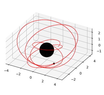
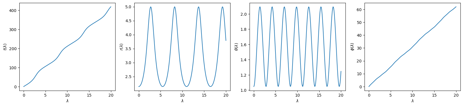
Next, compute the time, radial, polar and azimuthal components of the trajectory as a function of Mino time using the trajectory() method. By default, the time and radial components of the trajectory are given in geometrized units and are normalized using $M$ so that they are dimensionless.
t, r, theta, phi = orbit.trajectory()
import numpy as np
import matplotlib.pyplot as plt

time = np.linspace(0,20,200)

plt.figure(figsize=(20,4))

plt.subplot(1,4,1)
plt.plot(time, t(time))
plt.xlabel("$\lambda$")
plt.ylabel(r"$t(\lambda)$")

plt.subplot(1,4,2)
plt.plot(time, r(time))
plt.xlabel("$\lambda$")
plt.ylabel("$r(\lambda)$")

plt.subplot(1,4,3)
plt.plot(time, theta(time))
plt.xlabel("$\lambda$")
plt.ylabel(r"$\theta(\lambda)$")

plt.subplot(1,4,4)
plt.plot(time, phi(time))
plt.xlabel("$\lambda$")
plt.ylabel(r"$\phi(\lambda)$")
Orbital Properties
Use the constants_of_motion() method to compute the dimensionless energy, angular momentum and Carter constant. By default, constants of motion are given in geometrized units where $G=c=1$ and are scale-invariant, meaning that they are normalized according to the masses of the two bodies as follows:
$$ \mathcal{E} = \frac{E}{\mu}, \quad \mathcal{L} = \frac{L}{\mu M}, \quad \mathcal{Q} = \frac{Q}{\mu^2 M^2} $$
Here, $M$ is the mass of the primary body and $\mu$ is the mass of the secondary body.
Frequencies of motion can be computed in Mino time using the mino_frequencies() method and in Boyer-Lindquist time using the fundamental_frequencies() method. As with constants of motion, the frequencies returned by both methods are given in geometrized units and are normalized by $M$ so that they are dimensionless.
from IPython.display import display, Math

E, L, Q = orbit.constants_of_motion()

upsilon_r, upsilon_theta, upsilon_phi, gamma = orbit.mino_frequencies()

omega_r, omega_theta, omega_phi = orbit.fundamental_frequencies()


display(Math(fr"a = {orbit.a} \quad p = {orbit.p} \quad e = {orbit.e} \quad x = {orbit.x}"))

display(Math(fr"\mathcal{{E}} = {E:.3f} \quad \mathcal{{L}} = {L:.3f} \quad \mathcal{{Q}} = {Q:.3f}"))

display(Math(fr"""\Upsilon_r = {upsilon_r:.3f} \quad
             \Upsilon_\theta = {upsilon_theta:.3f} \quad
             \Upsilon_\phi = {upsilon_phi:.3f} \quad
             \Gamma = {gamma:.3f}"""))

display(Math(fr"""\Omega_r = {omega_r:.3f} \quad
            \Omega_\theta = {omega_theta:.3f} \quad
            \Omega_\phi = {omega_phi:.3f}"""))
$\displaystyle a = 0.999 \quad p = 3 \quad e = 0.4 \quad x = 0.8660254037844387$
$\displaystyle \mathcal{E} = 0.877 \quad \mathcal{L} = 1.903 \quad \mathcal{Q} = 1.265$
$\displaystyle \Upsilon_r = 1.145 \quad \Upsilon_\theta = 2.243 \quad \Upsilon_\phi = 3.118 \quad \Gamma = 20.531$
$\displaystyle \Omega_r = 0.056 \quad \Omega_\theta = 0.109 \quad \Omega_\phi = 0.152$
Plunging Orbits
Plunging orbits are parametrized using the spin parameter and the three constants of motion.
$a$ - spin of the primary body
$\mathcal{E}$ - Energy
$\mathcal{L}$ - $z$-component of angular momentum
$\mathcal{Q}$ - Carter constant
It is assumed that all orbital parameters are given in geometrized units where $G=c=1$ and are normalized according to the masses of the two bodies as follows:
$$ a = \frac{J}{M^2}, \quad \mathcal{E} = \frac{E}{\mu}, \quad \mathcal{L} = \frac{L}{\mu M}, \quad \mathcal{Q} = \frac{Q}{\mu^2 M^2} $$
Construct a PlungingOrbit by passing in these four parameters.
orbit = kg.PlungingOrbit(0.9, 0.94, 0.1, 12)
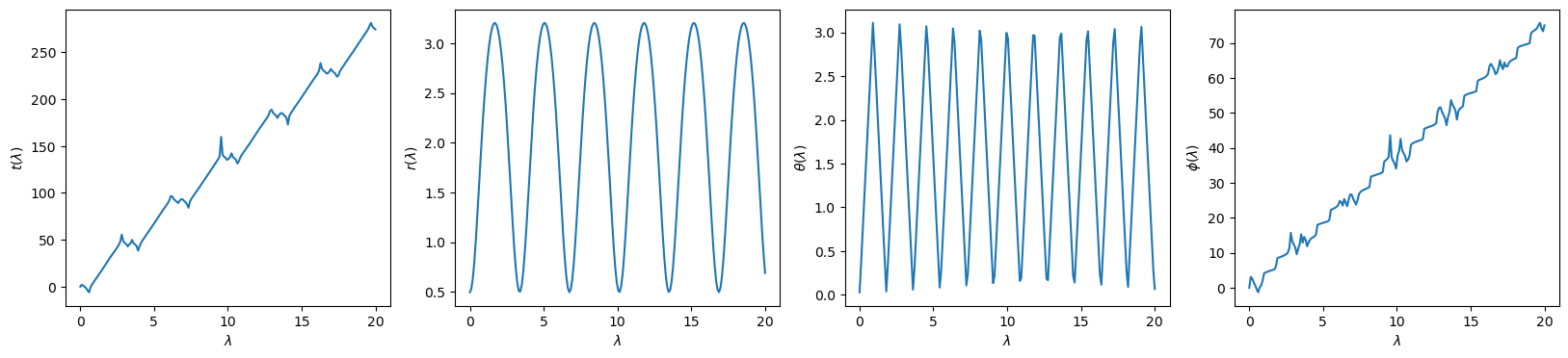
As with stable orbits, the components of the trajectory can be computed using the trajectory() method
t, r, theta, phi = orbit.trajectory()
import numpy as np
import matplotlib.pyplot as plt

time = np.linspace(0,20,200)

plt.figure(figsize=(20,4))

plt.subplot(1,4,1)
plt.plot(time, t(time))
plt.xlabel("$\lambda$")
plt.ylabel(r"$t(\lambda)$")

plt.subplot(1,4,2)
plt.plot(time, r(time))
plt.xlabel("$\lambda$")
plt.ylabel("$r(\lambda)$")

plt.subplot(1,4,3)
plt.plot(time, theta(time))
plt.xlabel("$\lambda$")
plt.ylabel(r"$\theta(\lambda)$")

plt.subplot(1,4,4)
plt.plot(time, phi(time))
plt.xlabel("$\lambda$")
plt.ylabel(r"$\phi(\lambda)$")
Alternative Parametrizations
Use the from_constants() class method to construct a StableOrbit from the spin parameter and constants of motion $(a,E,L,Q)$
orbit = kg.StableOrbit.from_constants(0.9, 0.95, 1.6, 8)
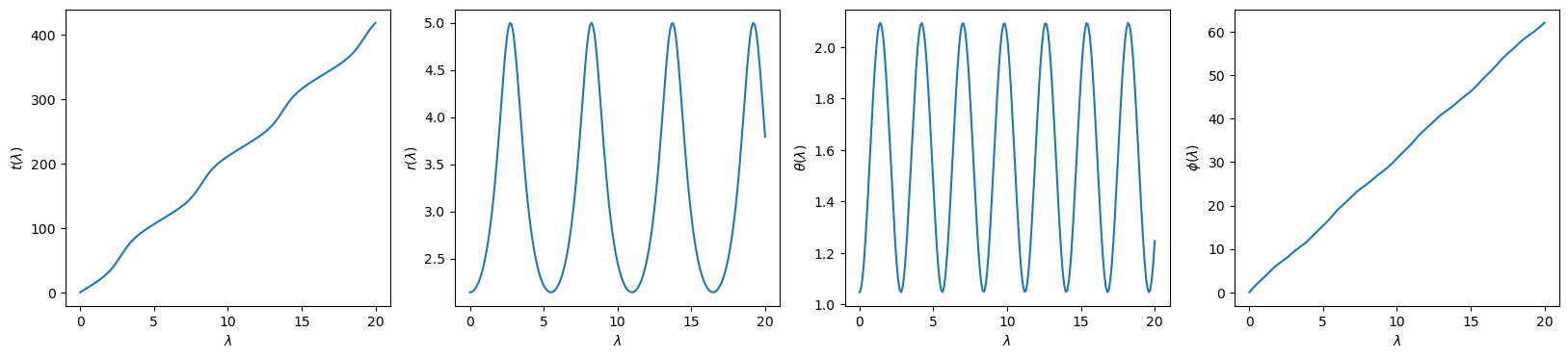
Use the Orbit class to construct an orbit from the spin parameter $a$, initial position $(t_0,r_0,\theta_0,\phi_0)$ and initial four-velocity $(u^t_0,u^r_0,u^{\theta}_0,u^{\phi}_0)$
stable_orbit = kg.StableOrbit(0.999,3,0.4,cos(pi/6))

x0 = stable_orbit.initial_position
u0 = stable_orbit.initial_velocity

orbit = kg.Orbit(0.999,x0,u0)
t, r, theta, phi = orbit.trajectory()

time = np.linspace(0,20,200)

plt.figure(figsize=(20,4))

plt.subplot(1,4,1)
plt.plot(time, t(time))
plt.xlabel("$\lambda$")
plt.ylabel(r"$t(\lambda)$")

plt.subplot(1,4,2)
plt.plot(time, r(time))
plt.xlabel("$\lambda$")
plt.ylabel("$r(\lambda)$")

plt.subplot(1,4,3)
plt.plot(time, theta(time))
plt.xlabel("$\lambda$")
plt.ylabel(r"$\theta(\lambda)$")

plt.subplot(1,4,4)
plt.plot(time, phi(time))
plt.xlabel("$\lambda$")
plt.ylabel(r"$\phi(\lambda)$")
Authors
- Seyong Park
- Zach Nasipak
1 maintainer

Metadata
1 maintainer
Release files for kerrgeopy 0.9.3
For a detailed explanation of source distributions (sdists) and built distributions (wheels), please see the package formats documentation.
Source distribution (sdist)
| File | Size | Uploaded | |
|---|---|---|---|
| kerrgeopy-0.9.3.tar.gz | 33.8 kB | Details |
Built distribution (wheel)
| File | Interpreter | ABI | Platform | Reset |
|---|---|---|---|---|
| kerrgeopy-0.9.3-py3-none-any.whl | Python 3 | none | any | Details |
Total release size: 67.9 kB
Release files / kerrgeopy-0.9.3.tar.gz
| Download URL | kerrgeopy-0.9.3.tar.gz |
|---|---|
| Size | 33.8 kB |
| Tags | Source |
|
SHA-256 checksum How to use checksums |
b046650906aaa364da3f4089a5289f14e1efa8f3b70dcd757b71b0c76b3c705e
|
|
BLAKE2b-256 checksum How to use checksums |
c2bdff0b54b2f3fc12c2635f64c1d82df5062b641767253bc02191d629dfad1f
|
| Upload date | |
|
Uploaded using Trusted Publishing? What is trusted publishing? |
No |
| Uploaded via |
twine/5.1.0 CPython/3.9.19
|
Release files / kerrgeopy-0.9.3-py3-none-any.whl
| Download URL | kerrgeopy-0.9.3-py3-none-any.whl |
|---|---|
| Size | 34.1 kB |
| Tags | Python 3 |
|
SHA-256 checksum How to use checksums |
87784b6864e257ef6e9f2c4d97f80fecc2c33f5547fa6511685019458cffb056
|
|
BLAKE2b-256 checksum How to use checksums |
549a5d9933ac1e0bc9028e6129c7ce6ffd0590a82bc804604c93decbe27387ba
|
| Upload date | |
|
Uploaded using Trusted Publishing? What is trusted publishing? |
No |
| Uploaded via |
twine/5.1.0 CPython/3.9.19
|














