No project description provided

Project description
knotted_graph: Analyzing Non-Hermitian Topological Nodal Structures


Figure: Non-Hermitian Nodal Phases — Exceptional Surface (lightgreen) and Exceptional Skeleton Graph (the graph within)
knotted_graph is a package designed to analyze and visualize the topological features of 2-band, 3-D non-Hermitian nodal systems. In these systems, the eigen-energies become complex, and points in momentum space where the Hamiltonian's eigenvalues and eigenvectors coalesce simultaneously are known as exceptional points (EPs).
In 3D non-Hermitian nodal systems, these EPs usually form an exceptional surfaces (ES). The skeleton (i.e. medial axis) serves as a topological fingerprint for the non-Hermitian nodal phase. The NodalSkeleton class helps in:
- Calculating the complex energy spectrum.
- Visualizing the 3D exceptional surface.
- Extracting the medial axis (skeleton) of the ES, which forms a spatial multigraph.
- Analyzing and visualizing the topology of this skeleton graph.
This guide will walk you through the process of using the NodalSkeleton class, from defining a Hamiltonian to analyzing its exceptional skeleton graph.
Installation
[!NOTE] The development is still in pre-alpha stage, expect bugs and rapid API changes.
You can install the package via pip:
$ pip install knotted_graph
or clone the repository and install it manually:
$ git clone https://github.com/sarinstein-yan/Nodal-Knot.git
$ cd Nodal-Knot
$ pip install -e .
This module is tested on Python >= 3.11.
Check the installation:
import knotted_graph as kg
print(kg.__version__)
Usage
Initializing the NodalSkeleton Class
- First, one needs to define a (non-interacting) 2-band non-Hermitian Hamiltonian in terms of the momentum vector $\vec{k} = (k_x, k_y, k_z)$.
The class accepts the Hamiltonian "Characteristic" in two forms:
- either as a 2x2
sympy.Matrix,
$$H(\vec{k}) = \vec{d}(\vec{k}) \cdot \vec{\sigma}$$
where $\vec{\sigma} = (\sigma_x, \sigma_y, \sigma_z)$ are the Pauli matrices,
- or directly as a tuple the components of the Bloch vector
(sympy.Expr, sympy.Expr, sympy.Expr):
$$\vec{d}(\vec{k}) = ( d_x(\vec{k}), d_y(\vec{k}), d_z(\vec{k}) )$$
The non-Hermiticity arises from complex terms in $\vec{d}(\vec{k})$.
-
Next, optionally, specify the k-space region of interest (the
spanparameter) and the resolution of the k-space grid (thedimensionparameter). -
If the $k$
sympysymbols in the input Hamiltoniansp.Matrixor(d_x, d_y, d_z)are named unconventionally, you need to specify them in thek_symbolsparameter. Otherwise, thek_symbolsare inferred from the input Hamiltoniancharacteristic.
Let's define a model that is known to produce a Hopf link nodal lines in the Hermitian limit. When the non-Hermiticity is introduced, the nodal line (exceptional line) will expand into a exceptional surface.
import numpy as np
import sympy as sp
from knotted_graph import NodalSkeleton

# Define momentum symbols
kx, ky, kz = sp.symbols('k_x k_y k_z', real=True)

# Use a non-Hermitian Bloch vector that can form a Hopf link
from knotted_graph.examples import hopf_link_bloch_vector

gamma = 0.1  # Non-Hermitian strength
d_x, d_y, d_z = hopf_link_bloch_vector(gamma)

# Initialize the `NodalSkeleton` with the Hamiltonian characteristic
ske = NodalSkeleton(
    char = (d_x, d_y, d_z),
    # k_symbols = (kx, ky, kz), # optional, we have named them *conventionally*
    # span = ((-np.pi, np.pi), (-np.pi, np.pi), (0, np.pi))
    # dimension = 200
)

print(f"Hamiltonian is Hermitian: {ske.is_Hermitian}")
print(f"Hamiltonian is PT-symmetric: {ske.is_PT_symmetric}")
>>>
Hamiltonian is Hermitian: False
Hamiltonian is PT-symmetric: False
Properties
- Hamiltonian matrix (
sympy.Matrix):
ske.h_k
>>>
$$\left[\begin{matrix}(2 \cos{(2 k_{z})} + 1) (\cos{(k_{x})} + \cos{(k_{y})} + \cos{(k_{z})} - 2) - 2 \sin{(k_{x})} \sin{(k_{y})} & \frac{(2 \cos{(2 k_{z})} + 1)^{2}}{4} - (\cos{(k_{x})} + \cos{(k_{y})} + \cos{(k_{z})} - 2)^{2} - \sin^{2}{(k_{x})} + \sin^{2}{(k_{y})} + 0.1 \\ \frac{(2 \cos{(2 k_{z})} + 1)^{2}}{4} - (\cos{(k_{x})} + \cos{(k_{y})} + \cos{(k_{z})} - 2)^{2} - \sin^{2}{(k_{x})} + \sin^{2}{(k_{y})} - 0.1 & - (2 \cos{(2 k_{z})} + 1) (\cos{(k_{x})} + \cos{(k_{y})} + \cos{(k_{z})} - 2) + 2 \sin{(k_{x})} \sin{(k_{y})}\end{matrix}\right]$$
- Bloch vector (
(sp.Expr, sp.Expr, sp.Expr)):
ske.bloch_vec
>>>
((2*cos(2*k_z) + 1)**2/4 - (cos(k_x) + cos(k_y) + cos(k_z) - 2)**2 - sin(k_x)**2 + sin(k_y)**2,
 0.1*I,
 (2*cos(2*k_z) + 1)*(cos(k_x) + cos(k_y) + cos(k_z) - 2) - 2*sin(k_x)*sin(k_y))
- $k$-space region information:
print(f"self.dimension: {ske.dimension}")
print(f"self.spacing: {ske.spacing}")
print(f"self.origin: {ske.origin}")

print(f"self.span: {ske.span}")
print(f"self.kx_span: {ske.kx_span}")
print(f"self.ky_span: {ske.ky_span}")
print(f"self.kz_span: {ske.kz_span}")

# Below attributes are also available for y and z
print(f"self.kx_min: {ske.kx_min}")
print(f"self.kx_max: {ske.kx_max}")
print(f"self.kx_symbol: {ske.kx_symbol} | {type(ske.kx_symbol)}")
print(f"self.kx_vals: shape - {ske.kx_vals.shape} | dtype - {ske.kx_vals.dtype}")
print(f"self.kx_grid: shape - {ske.kx_grid.shape} | dtype - {ske.kx_grid.dtype}")
>>>
self.dimension: 200
self.spacing: [0.0315738 0.0315738 0.0157869]
self.origin: [-3.14159265 -3.14159265  0.        ]
self.span: [[-3.14159265  3.14159265]
 [-3.14159265  3.14159265]
 [ 0.          3.14159265]]
self.kx_span: (-3.141592653589793, 3.141592653589793)
self.ky_span: (-3.141592653589793, 3.141592653589793)
self.kz_span: (0, 3.141592653589793)
self.kx_min: -3.141592653589793
self.kx_max: 3.141592653589793
self.kx_symbol: k_x | <class 'sympy.core.symbol.Symbol'>
self.kx_vals: shape - (200,) | dtype - float64
self.kx_grid: shape - (200, 200, 200) | dtype - float64
- Energy spectrum (only the upper band) (
np.ndarray):
ske.spectrum.shape, ske.spectrum.dtype
>>>
((200, 200, 200), dtype('complex128'))
- Band gap (=
2 × |upper band spectrum|) (np.ndarray):
ske.band_gap.shape, ske.band_gap.dtype
>>>
((200, 200, 200), dtype('float64'))
Skeleton graph (networkx.MultiGraph):
graph = ske.skeleton_graph(
    # simplify = True,  # Topological simplification
    # smooth_epsilon = 4,  # Smoothness, unit is pixel
    # skeleton_image = ... # Can construct a skeleton graph from an skeletonized image
)
graph
>>>
<networkx.classes.multigraph.MultiGraph at 0x26d8b529b80>
- Check if the graph is trivalent
I.e. whether each vertex has degree <= 3. If trivalent, the Yamada polynomial is an isotopic invariant of the skeleton multigraph.
graph.graph['is_trivalent']
>>>
(True, True)
- Graph summary:
ske.graph_summary()
>>>
| Property               | Value   |
|------------------------|---------|
| Number of nodes        | 2       |
| Number of edges        | 2       |
| Connected              | No      |
| # Connected components | 2       |
| Component 1 size       | 1       |
| Component 2 size       | 1       |

Degree distribution:
|   Degree |   Frequency |
|----------|-------------|
|        2 |           2 |
- Check graph minors:
import networkx as nx

# Check if K_3 graph (a cycle of 3 nodes) is a minor of our skeleton graph
k3_graph = nx.complete_graph(3)
print("Checking for K3 minor...")
ske.check_minor(minor_graph=k3_graph)

# Now, let's try a more complex graph, K4 (complete graph of 4 nodes)
# A simple loop shouldn't contain a K4 minor.
k4_graph = nx.complete_graph(4)
print("\nChecking for K4 minor...")
ske.check_minor(k4_graph, host_graph=graph)
>>>
Checking for K3 minor...
The given graph DOES NOT contain the minor graph.

Checking for K4 minor...
The given graph DOES NOT contain the minor graph.
Visualization
NodalSkeleton uses pyvista for 3D plotting, creating interactive visualizations.
Plotting the Exceptional Surface
The exceptional surface is the 3D surface in k-space where the band gap closes, defined by $$ |d(\vec{k})| = 0 \Leftrightarrow d_x(\vec{k})^2 + d_y(\vec{k})^2 + d_z(\vec{k})^2 = 0 $$
The code cells below are meant to be run in a Jupyter notebook.
import pyvista as pv
pv.set_jupyter_backend('client')
EXPORT_FIGS = True  # Set to True to export figures

plotter = ske.plot_exceptional_surface()
plotter.add_bounding_box()
plotter.show()
if EXPORT_FIGS:
    plotter.export_html(f'./assets/ES_gamma={gamma}.html')
    plotter.save_graphic(f'./assets/ES_gamma={gamma}.svg')
    plotter.save_graphic(f'./assets/ES_gamma={gamma}.pdf')

Click here to view the interactive 3D plot
To add projected silhouettes of the exceptional surface onto the Surface Brillouin Zone (SBZ) planes, set add_silhouettes=True:
plotter = ske.plot_exceptional_surface(
    add_silhouettes=True,  # Add projected silhouettes onto the SBZ planes
    silh_origins=np.diag([-np.pi, -np.pi, 0]),
    # ^ Origin of the planes that the silhouettes are projected onto
)
plotter.show_bounds(xtitle='kx', ytitle='ky', ztitle='kz')
plotter.add_bounding_box()
plotter.zoom_camera(1.2)
plotter.show()
if EXPORT_FIGS:
    plotter.export_html(f'./assets/ES_gamma={gamma}_silhouettes.html')
    plotter.save_graphic(f'./assets/ES_gamma={gamma}_silhouettes.svg')
    plotter.save_graphic(f'./assets/ES_gamma={gamma}_silhouettes.pdf')

Click here to view the interactive 3D plot
Plotting the Exceptional Skeleton Graph
The exceptional skeleton graph is the medial axis of the exceptional surface interior, where the energy spectrum is purely imaginary.
plotter = ske.plot_skeleton_graph(
    add_nodes=False, # since the skeleton is essentially a Hopf link
    add_silhouettes=True,
    silh_origins=np.diag([-np.pi, -np.pi, 0]),
)
plotter.show_bounds(xtitle='kx', ytitle='ky', ztitle='kz')
plotter.add_bounding_box()
plotter.show()
if EXPORT_FIGS:
    plotter.export_html(f'./assets/SG_gamma={gamma}_silhouettes.html')
    plotter.save_graphic(f'./assets/SG_gamma={gamma}_silhouettes.svg')
    plotter.save_graphic(f'./assets/SG_gamma={gamma}_silhouettes.pdf')

Click here to view the interactive 3D plot
Non-Hermiticity induced exceptional knotted graph
For nodal knot systems, in the Hermitian limit or when non-Hermitian perturbation is small, the original knot / link topology is preserved, as shown above (gamma=0.1).
When non-Hermiticity is prevalent enough, the exceptional surface starts to touch itself, leading to topological transitions --- the skeleton (i.e., medial axis) of the exceptional surface becomes a knotted graph (a.k.a. spatial multigraph).
As the non-Hermiticity evolves, the knotted graph topology evolves accordingly, leading to a plethora of exotic 3D spatial geometries in the momentum space.
E.g., let us set gamma = [0.2, 0.5]:
for gamma in [0.2, 0.5]:
    print(f"With gamma = {gamma}:\n")

    ske_ = NodalSkeleton(hopf_bloch_vector(gamma))
    ske_.graph_summary(ske.skeleton_graph())

    plotter = ske_.plot_exceptional_surface(surf_opacity=.3, surf_color='lightgreen')
    plotter = ske_.plot_skeleton_graph(plotter=plotter)

    if EXPORT_FIGS:
        plotter.export_html(f'./assets/ES_SG_gamma={gamma}.html')
        plotter.save_graphic(f'./assets/ES_SG_gamma={gamma}.svg')
        plotter.save_graphic(f'./assets/ES_SG_gamma={gamma}.pdf')
        plotter.show()
>>>
With gamma = 0.2:

| Property          | Value              |
|-------------------|--------------------|
| Number of nodes   | 4                  |
| Number of edges   | 6                  |
| Connected         | Yes                |
| Diameter          | 2                  |
| Avg shortest path | 1.3333333333333333 |

Degree distribution:
|   Degree |   Frequency |
|----------|-------------|
|        3 |           4 |

Click here to view the interactive 3D plot
With gamma = 0.5:

| Property          | Value   |
|-------------------|---------|
| Number of nodes   | 2       |
| Number of edges   | 3       |
| Connected         | Yes     |
| Diameter          | 1       |
| Avg shortest path | 1.0     |

Degree distribution:
|   Degree |   Frequency |
|----------|-------------|
|        3 |           2 |

Click here to view the interactive 3D plot
Planar Diagram and Yamada Polynomial
If a skeleton graph is trivalent (all node degrees <= 3), the Yamada polynomial is an isotopic invariant of the spatial graph.
If not trivalent, the Yamada polynomial is still well-defined, but it is not an isotopic invariant, but rather a rigid isotopy invariant --- it depends on how one projects the 3D skeleton graph onto a 2D plane.
For a trivalent skeleton graph, NodalSkeleton.yamada_polynomial(variable) by default will sample num_rotations=10 different projections that quotient out the rotational symmetry that produces the same planar diagram, and start from the planar diagram with the least number of crossings.
If it finds two Yamada polynomials agree, which usually happens right after computing from the best two projections, it will return the agreed Yamada polynomial.
If after num_rotations computations, no two Yamada polynomials agree, it will return the projection data and the corresponding Yamada polynomials.
# define the variable of the Yamada polynomial
A = sp.symbols('A')

_ = ske.skeleton_graph() # Ensure the skeleton graph is computed and cached
print("Is the skeleton graph trivalent?", ske.is_graph_trivalent)

# Compute the Yamada polynomial for the Hopf Link
Y = ske.yamada_polynomial(
    variable=A,
    # normalize=True, # Normalize the Yamada polynomial
    # n_jobs=-1, # Use all available cores for one view

    num_rotations=10, # ONLY for trivalent graphs

    # rotation_angles=(0., 0., 0.), # ONLY for non-trivalent graphs
    # rotation_order='ZYX' # ONLY for non-trivalent graphs
)
Y
>>>
Is the skeleton graph trivalent? True
Computing Yamada polynomial:  10%|█         | 1/10 [00:00<00:01,  5.72it/s]
$$- A^{7} - A^{6} - A^{5} + A^{3} + 2 A^{2} + 2 A + 1$$
There a few ways to compute the Yamada polynomial apart from the NodalSkeleton.yamada_polynomial() method.
E.g., by a function call:
kg.compute_yamada_safely(
    skeleton_graph=hopf_link,
    variable=A,
    # num_rotations=10,
    # normalize=True,
    # n_jobs=-1
)
>>>
Computing Yamada polynomial: 10%|█ | 1/10 [00:00<00:01, 5.72it/s]
$$- A^{7} - A^{6} - A^{5} + A^{3} + 2 A^{2} + 2 A + 1$$
Or from the planar diagram code:
pd = kg.PDCode(skeleton_graph=hopf_link)

pd_code = pd.compute(
    # specify the projection angles and order if needed
    rotation_angles=(137.5, 81.4, 0.),
    # rotation_order='ZYX',
)
print(f"planar diagram code: {pd_code}")

pd.compute_yamada(A, normalize=True)
>>>
planar diagram code: V[0,2];V[3,5];X[4,1,3,2];X[4,0,5,1]
$$- A^{7} - A^{6} - A^{5} + A^{3} + 2 A^{2} + 2 A + 1$$
Or from a thinly wrapped function:
kg.compute_yamada_polynomial(hopf_link, A, (137.5, 81.4, 0.))
>>>
$$- A^{7} - A^{6} - A^{5} + A^{3} + 2 A^{2} + 2 A + 1$$
For a non-trivalent skeleton graph, the NodalSkeleton.yamada_polynomial(variable) will only compute from one projection, specified by the
rotation_angles[=(0., 0., 0.)] and rotation_order[='ZYX']
parameters (see NodalSkeleton.util.get_rotation_matrix for the meaning of these parameters).
One can call knotted_graph.util.generate_isotopy_projections to generate a list of projections sorted by the number of crossings in the planar diagram, and then call NodalSkeleton.yamada_polynomial(variable, rotation_angles=best_proj['angles']) to compute the Yamada polynomial from the best projection.
projections = kg.generate_isotopy_projections(
    skeleton_graph=hopf_link,
    num_rotations=10
)

best_proj = projections[0]
print(f"Keys of a projection: {best_proj.keys()}")
print(f"Number of crossings: {best_proj['num_crossings']}")
print(f"Angles: {best_proj['angles']}")
print(f"pd_code: {best_proj['pd_code']}")

kg.compute_yamada_polynomial(hopf_link, A, best_proj['angles'])
# Or `ske.yamada_polynomial(variable=A, rotation_angles=best_proj['angles'])`
>>>
Keys of a projection: dict_keys(['num_crossings', 'vertices', 'crossings', 'arcs', 'angles', 'pd_code'])
Number of crossings: 2
Angles: [0.0, 87.13401601740115, 0.0]
pd_code: V[0,2];V[3,5];X[2,4,1,3];X[4,0,5,1]
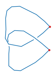
Visualization of the planar diagram
NodalSkeleton.plot_planar_diagram can be used to visualize the planar diagram of a given rotation angle for projection.
import matplotlib.pyplot as plt

fig, ax = plt.subplots(figsize=(3,3))
ax = ske.plot_planar_diagram(
    ax = ax,
    rotation_angles = projections[0]['angles'],
    # rotation_order = 'ZYX',
    # undercrossing_offset = 5.
    # mark_crossings = False
)
ax.set_aspect('equal')
ax.axis('off')
if EXPORT_FIGS:
    plt.savefig("./assets/planar_diagram.png", bbox_inches='tight')
plt.show()
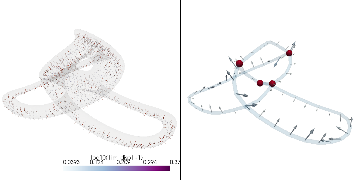
Physical Fields Visualization
One can plot physical vector / scalar fields within the Exceptional Surface or on the Skeleton Graph edges.
Fields data are stored in the property NodalSkeleton.fields_pv as a pyvista.ImageData
bvec = kg.hopf_link_bloch_vector(.4, (kx, ky, kz))
ske = kg.NodalSkeleton(bvec)

ske.fields_pv
Energy Dispersion $\nabla_{\vec{k}}\text{Im}(E)$
pl = pv.Plotter(shape=(1, 2), window_size=[1200, 600])
pl.subplot(0, 0)
pl = ske.plot_interior_dispersion(pl, glyph_factor=0.1, glyph_tolerance=0.015)
pl.subplot(0, 1)
pl = ske.plot_skeleton_graph(pl, add_edge_field=True,
                             orient='im_disp', scale='log10(|im_disp|+1)',
                             field_cmap='BuPu', glyph_factor=1.2)
pl.link_views()
pl.camera_position = [[-0.75, -7.62, 3.67], [0.14, -0.08, 0.96], [0.01, 0.34, 0.94]]
if EXPORT_FIGS:
    pl.screenshot("./assets/field_dispersion.png")
pl.show()
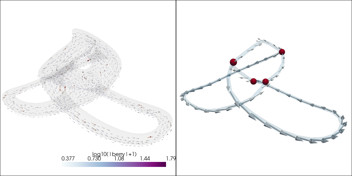
Berry Curvature $\vec{\Omega} := \nabla_{\vec{k}} \times \vec{A}$
$\vec{A} := \text{Re}(i \left< \phi^L | \nabla_{\vec{k}} | \phi^R \right> )$ is the Berry connection.
pl = pv.Plotter(shape=(1, 2), window_size=[1200, 600])
pl.subplot(0, 0)
pl = ske.plot_berry_curvature(pl, glyph_factor=0.03, glyph_tolerance=0.015)
pl.subplot(0, 1)
pl = ske.plot_skeleton_graph(pl, add_edge_field=True,
                             orient='berry', scale='log10(|berry|+1)',
                             field_cmap='BuPu', glyph_factor=.3)
pl.link_views()
pl.camera_position = [[-0.75, -7.62, 3.67], [0.14, -0.08, 0.96], [0.01, 0.34, 0.94]]
if EXPORT_FIGS:
    pl.screenshot("./assets/field_berry.png")
pl.show()
Custom Visualization
One can add custom vector / scalar field data.
E.g. here we add the gradient of the Im(E) and the gradient of Berry curvature magnitude.
vol = ske.fields_pv.copy()
# add extra fields
vol = vol.compute_derivative(scalars='|berry|', gradient='∇|berry|')
vol.point_data['log10(|∇|berry||+1)'] = - np.log10( np.linalg.norm(vol.point_data['∇|berry|'], axis=-1) +1)
vol = vol.compute_derivative(scalars='|im_disp|', gradient='∇|im_disp|')
vol.point_data['log10(|∇|im_disp||+1)'] = - np.log10( np.linalg.norm(vol.point_data['∇|im_disp|'], axis=-1) +1)

vol
Visualizing the iso-surfaces of scalar fields with pyvista interactive widgets.
scalars = ['imag',
           'log10(|berry|+1)', 'log10(|im_disp|+1)',
           '|berry|', '|im_disp|',
           'log10(|∇|berry||+1)', 'log10(|∇|im_disp||+1)']

# null out the exterior points
mask = np.where(vol.point_data['imag'] == 0)
for s in scalars:
    vol.point_data[s][mask] = np.nan

pv.set_jupyter_backend('trame')
pl2 = pv.Plotter(window_size=(800, 600))
ske.plot_exceptional_surface(pl2, surf_opacity=0.05, surf_color='gray')
pl2.add_mesh_isovalue(vol, scalars=scalars[0], opacity=0.5, cmap='BuPu')
pl2.add_legend()
pl2.add_bounding_box()
pl2.show()
TODO:
- Documentation website
- Graph diagram visualization with parallel projection
- Batched processing. Move the spectrum calculation batch to GPU.
- Multi-band Hamiltonians support
Project details
Release history Release notifications | RSS feed


Download files
Download the file for your platform. If you're not sure which to choose, learn more about installing packages.
Source Distribution
Built Distribution
Filter files by name, interpreter, ABI, and platform.
If you're not sure about the file name format, learn more about wheel file names.
Copy a direct link to the current filters
File details
Details for the file knotted_graph-0.1.1.tar.gz.
File metadata
- Download URL: knotted_graph-0.1.1.tar.gz
- Upload date:
- Size: 44.6 kB
- Tags: Source
- Uploaded using Trusted Publishing? No
- Uploaded via: python-httpx/0.28.1
File hashes
| Algorithm | Hash digest | |
|---|---|---|
| SHA256 |
716eefcc9f82a426cf6a5c6bc6495fa71fac0e6c309327f3de323e090dab59aa
|
|
| MD5 |
d5221144eee73e7dd3c120c880fae35e
|
|
| BLAKE2b-256 |
202125b06bb72d11de05c3ee02093f872041e0aaee9e4d59197af3960b71c70d
|
File details
Details for the file knotted_graph-0.1.1-py3-none-any.whl.
File metadata
- Download URL: knotted_graph-0.1.1-py3-none-any.whl
- Upload date:
- Size: 48.6 kB
- Tags: Python 3
- Uploaded using Trusted Publishing? No
- Uploaded via: python-httpx/0.28.1
File hashes
| Algorithm | Hash digest | |
|---|---|---|
| SHA256 |
b50f8ead9a862492999c0629633e1b899ec20fb2f3e5029fd756765dd905a68b
|
|
| MD5 |
a16712b6e6d46aa798b8cbfbd492c5a9
|
|
| BLAKE2b-256 |
78ff191d2b837a7482bf83f8fb096b093740770d0ab2c56459b593fc1bd5b03f
|


