
KurveRSC
KurveRSC is an integrated relational representation and model-selection system. It uses GraphReduce as its relational feature engine, searches graph configurations across temporal frames, and selects them by downstream validation performance.
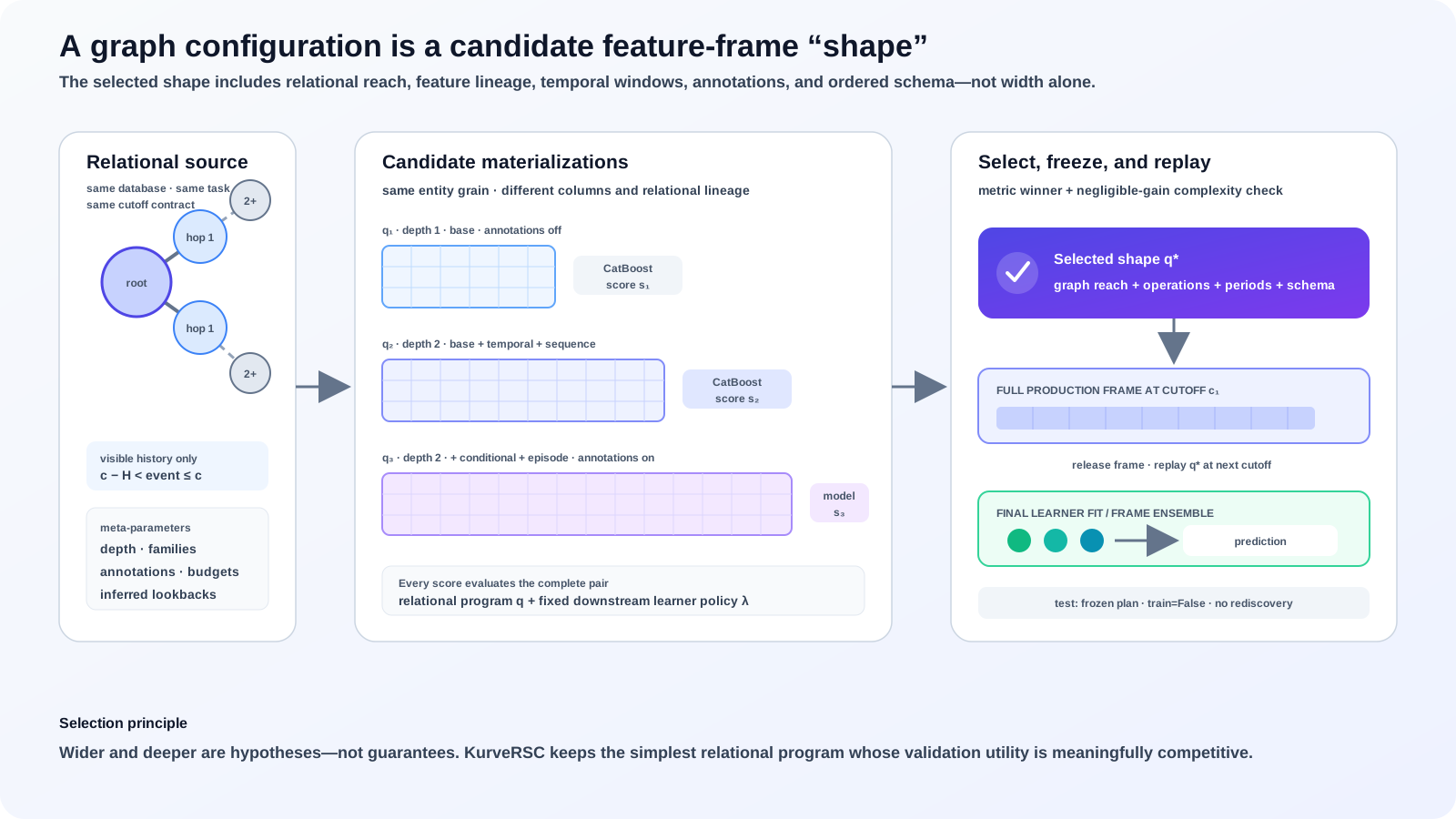
KurveRSC searches the relational signal-compression space and fits the selected shape on full point-in-time data.
Thesis. Relational signal compression is a first-class optimization surface. Long-term progress will come not only from improving the downstream learner, but from learning which paths, time windows, reductions, and feature families should carry a database's task-relevant signal into that learner. Keeping this boundary explicit makes the learner pluggable: today CatBoost; tomorrow TabPFN-3 or another tabular or relational foundation model.
Two independent results motivate this direction. KumoRFM-2 reports that task-specific fine-tuning improves its average SALT MRR from 0.83 in-context to 0.89, showing that a strong relational foundation model still benefits materially from task adaptation (KumoRFM-2). Prior Labs' TabPFN-Rel couples Deep Feature Synthesis with TabPFN-3 and obtains leading RelArena results, showing that a foundation learner can benefit from a separately constructed relational representation (RelArena and TabPFN-Rel). These systems do not optimize the same object as KurveRSC, but together support its modular hypothesis: relational representation and downstream learning should be adapted jointly without permanently binding either layer to the other.
How KurveRSC differs from Deep Feature Synthesis
Deep Feature Synthesis generates a relational feature space; KurveRSC selects a relational program by measuring how well its complete feature frame works with the downstream learner.
| Dimension | Deep Feature Synthesis | GraphReduce | KurveRSC |
|---|---|---|---|
| Primary object | Composed feature definitions | Executable table graph and node operations | Search over complete GraphReduce programs |
| Learner role | Normally fitted after synthesis | External to the execution engine | In the loop: AUROC or MAE scores every candidate frame |
| Task adaptation | Caller chooses primitives and depth; later feature selection can remove columns | Caller configures one graph program | Search jointly chooses depth, families, annotations, budgets, and temporal policy |
| Final artifact | Feature definitions and materialized table | Reduced frame and operation lineage | Selected configuration, frozen execution plan, schema, and fitted learner |
| Inference | Recompute the chosen definitions | Re-execute the configured graph | Replay the learned plan with feature discovery disabled |
Learner regularization over a wide DFS matrix can choose among columns that were generated, but it cannot recover paths, time windows, feature families, or propagation depths that were never materialized. KurveRSC makes those upstream choices part of validation-guided selection while retaining a replaceable downstream model. See the technical report's full comparison.
The KurveRSC technical report (PDF) explains the GraphReduce algorithm, relational feature families, learner-guided graph search, point-in-time guarantees, frozen-plan lifecycle, and evaluation protocol. The shorter Kurve RSC white paper (PDF) introduces the central optimization idea.
Quickstart
The high-level API is one function. Give fit an entity table, a label table,
their join keys, the target, and an authoritative train/validation split:
pip install "kurversc[relbench]" # omit [relbench] for ordinary tables
import kurversc

result = kurversc.fit(
    parent_node="customers.parquet",
    label_node="churn_labels.parquet",
    parent_key="customer_id",
    label_key="customer_id",
    target="churn",
    split_column="split",  # values: train / validation
)

print(result.best_config)         # highest validation ROC AUC or lowest MAE
print(result.recommended_config)  # simpler config when the gain is negligible
print(result.full_validation_score)
print(result.results)             # complete configuration-search audit trail
result is the fitted KurveRSC artifact: the selected GraphConfig, frozen
GraphReduce feature-operation plan, downstream learner, feature schema, and
validation metadata. Pass it to kurversc.predict(...) to replay the exact
learned relational program at new cutoff dates.
RelArena performance
The September 1, 2026 reference profile uses official RelBench v1 test splits through RelArena: full-data latest-cutoff graph search, three sequential reranking folds, one production cutoff, CatBoost, GraphReduce's fixed temporal periods, and no automatic text features. Classification reports test AUROC (higher is better); regression reports test MAE (lower is better).
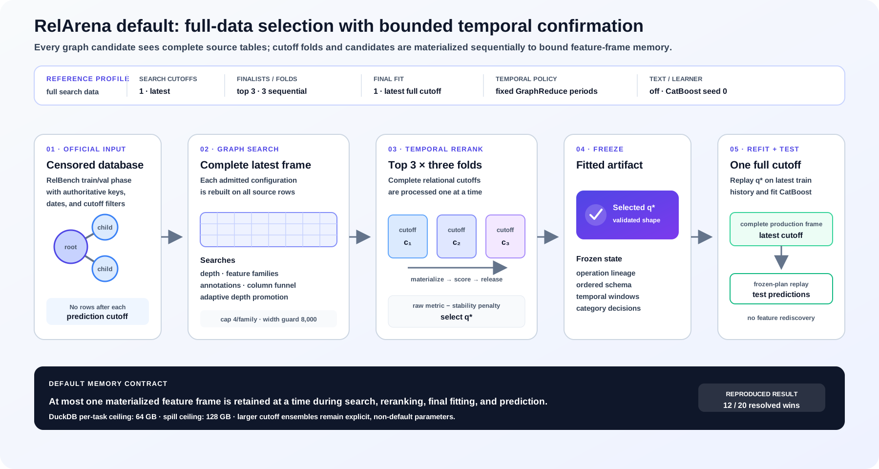
The reported reproducibility default prioritizes complete graph-configuration evidence while retaining only one materialized feature frame at a time.
| Dataset | Task | Metric | KurveRSC | TabPFN-Rel Local | Winner |
|---|---|---|---|---|---|
| rel-amazon | user-churn | AUROC ↑ | 0.709790 | 0.702403 | KurveRSC |
| rel-amazon | item-churn | AUROC ↑ | 0.828114 | 0.827857 | KurveRSC |
| rel-amazon | user-ltv | MAE ↓ | 14.132556 | 14.400940 | KurveRSC |
| rel-amazon | item-ltv | MAE ↓ | 42.205991 | 47.768328 | KurveRSC |
| rel-avito | user-visits | AUROC ↑ | 0.674295 | 0.668811 | KurveRSC |
| rel-avito | user-clicks | AUROC ↑ | 0.654236 | 0.614522 | KurveRSC |
| rel-avito | ad-ctr | MAE ↓ | 0.033654 | 0.031379 | TabPFN-Rel Local |
| rel-event | user-repeat | AUROC ↑ | 0.780414 | 0.769251 | KurveRSC |
| rel-event | user-ignore | AUROC ↑ | 0.830661 | 0.701376 | KurveRSC |
| rel-event | user-attendance | MAE ↓ | 0.258185 | 0.239383 | TabPFN-Rel Local |
| rel-f1 | driver-dnf | AUROC ↑ | 0.753628 | 0.714468 | KurveRSC |
| rel-f1 | driver-top3 | AUROC ↑ | 0.673136 | 0.792916 | TabPFN-Rel Local |
| rel-f1 | driver-position | MAE ↓ | 3.913762 | 3.761699 | TabPFN-Rel Local |
| rel-hm | user-churn | AUROC ↑ | 0.696866 | 0.705690 | TabPFN-Rel Local |
| rel-hm | item-sales | MAE ↓ | 0.032107 | 0.061362 | KurveRSC |
| rel-stack | user-engagement | AUROC ↑ | 0.903450 | 0.905834 | TabPFN-Rel Local |
| rel-stack | user-badge | AUROC ↑ | 0.877852 | 0.863470 | KurveRSC |
| rel-stack | post-votes | MAE ↓ | 0.063347 | 0.067957 | KurveRSC |
| rel-trial | study-outcome | AUROC ↑ | 0.704273 | 0.730607 | TabPFN-Rel Local |
| rel-trial | study-adverse | MAE ↓ | 42.024547 | 42.591708 | KurveRSC |
| rel-trial | site-success | MAE ↓ | 0.402717 | 0.385751 | TabPFN-Rel Local |
KurveRSC wins 13 of 21 direct comparisons with TabPFN-Rel Local: 8–4 on classification and 5–4 on regression. On the complete 21-task matrix it is third overall by RelArena's bootstrapped Elo calculation at 1786.7, behind RT-PluRel and TabPFN-Rel API and ahead of TabPFN-Rel Local.
Aggregate RelArena leaderboard
This table includes every reproduced RelArena participant on the complete 21-task matrix. Elo is anchored to the global constant predictor at 1000; higher Elo and win rate are better, while lower mean rank and rescaled loss are better.
| Elo rank | Method | Kind | Elo | Mean rank | Win rate | Rescaled loss |
|---|---|---|---|---|---|---|
| 1 | RT-PluRel | system | 1858.7 | 2.952 | 80.48% | 0.107752 |
| 2 | TabPFN-Rel API | model | 1824.0 | 3.286 | 77.14% | 0.148825 |
| 3 | KurveRSC | system | 1786.7 | 3.667 | 73.33% | 0.142977 |
| 4 | TabPFN-Rel Local | model | 1725.5 | 4.333 | 66.67% | 0.190129 |
| 5 | GraphSAGE | model | 1663.0 | 5.048 | 59.52% | 0.207151 |
| 6 | RelGT | model | 1578.7 | 6.024 | 49.76% | 0.321981 |
| 7 | RDBLearn | model | 1564.1 | 6.190 | 48.10% | 0.274366 |
| 8 | RelGNN-ES | model | 1528.0 | 6.595 | 44.05% | 0.306010 |
| 9 | LightGBM (entity-only) | model | 1359.8 | 8.286 | 27.14% | 0.546964 |
| 10 | Constant (per-entity) | model | 1259.5 | 9.095 | 19.05% | 0.618485 |
| 11 | Constant (global) | model | 1000.0 | 10.524 | 4.76% | 0.941953 |
Ranking by rescaled loss
RelArena's default aggregate orders methods by mean per-task min-max rescaled error. Lower is better; the Elo rank is retained to make the two orderings easy to compare.
| Loss rank | Method | Kind | Rescaled loss | Elo rank | Elo |
|---|---|---|---|---|---|
| 1 | RT-PluRel | system | 0.107752 | 1 | 1858.7 |
| 2 | KurveRSC | system | 0.142977 | 3 | 1786.7 |
| 3 | TabPFN-Rel API | model | 0.148825 | 2 | 1824.0 |
| 4 | TabPFN-Rel Local | model | 0.190129 | 4 | 1725.5 |
| 5 | GraphSAGE | model | 0.207151 | 5 | 1663.0 |
| 6 | RDBLearn | model | 0.274366 | 7 | 1564.1 |
| 7 | RelGNN-ES | model | 0.306010 | 8 | 1528.0 |
| 8 | RelGT | model | 0.321981 | 6 | 1578.7 |
| 9 | LightGBM (entity-only) | model | 0.546964 | 9 | 1359.8 |
| 10 | Constant (per-entity) | model | 0.618485 | 10 | 1259.5 |
| 11 | Constant (global) | model | 0.941953 | 11 | 1000.0 |
KurveRSC is also second overall by rescaled loss, behind RT-PluRel. Because systems use their own internal selection regimes, RelArena reports method kind explicitly: KurveRSC and RT-PluRel are systems, while the remaining learned participants are models under RelArena's standardized tuning interface.
Per-task results across all participants
These matrices combine KurveRSC's default-profile test results with the validation-selected, seed-zero test scores in RelArena's reproduced release artifact. Bold marks the best held-out score on each task. AUROC is maximized; MAE is minimized.
Classification — AUROC ↑
| Dataset / task | KurveRSC | RT-PluRel | TabPFN-Rel API | TabPFN-Rel Local | GraphSAGE | RelGT | RDBLearn | RelGNN-ES | LightGBM | Constant/entity | Constant/global | Overall winner |
|---|---|---|---|---|---|---|---|---|---|---|---|---|
| rel-amazon/item-churn | 0.828114 | 0.832656 | 0.827996 | 0.827857 | 0.830527 | 0.823835 | 0.819538 | 0.785579 | 0.662211 | 0.728875 | 0.500000 | RT-PluRel |
| rel-amazon/user-churn | 0.709790 | 0.713460 | 0.708649 | 0.702403 | 0.704596 | 0.701924 | 0.684375 | 0.694281 | 0.517056 | 0.634205 | 0.500000 | RT-PluRel |
| rel-avito/user-clicks | 0.654236 | 0.583376 | 0.675191 | 0.614522 | 0.608674 | 0.644353 | 0.678769 | 0.667571 | 0.564163 | 0.504143 | 0.500000 | RDBLearn |
| rel-avito/user-visits | 0.674295 | 0.670887 | 0.668026 | 0.668811 | 0.665758 | 0.662142 | 0.659624 | 0.648731 | 0.529282 | 0.602703 | 0.500000 | KurveRSC |
| rel-event/user-ignore | 0.830661 | 0.847577 | 0.878659 | 0.701376 | 0.758728 | 0.781507 | 0.664351 | 0.805393 | 0.777181 | 0.839930 | 0.500000 | TabPFN-Rel API |
| rel-event/user-repeat | 0.780414 | 0.791377 | 0.759291 | 0.769251 | 0.784626 | 0.734358 | 0.744084 | 0.754612 | 0.748295 | 0.751805 | 0.500000 | RT-PluRel |
| rel-f1/driver-dnf | 0.753628 | 0.731460 | 0.732172 | 0.714468 | 0.717235 | 0.711667 | 0.714551 | 0.726106 | 0.730298 | 0.699258 | 0.500000 | KurveRSC |
| rel-f1/driver-top3 | 0.673136 | 0.758858 | 0.771426 | 0.792916 | 0.725975 | 0.810841 | 0.780081 | 0.758864 | 0.738889 | 0.556530 | 0.500000 | RelGT |
| rel-hm/user-churn | 0.696866 | 0.704356 | 0.705215 | 0.705690 | 0.698525 | 0.689531 | 0.698352 | 0.682025 | 0.590081 | 0.647972 | 0.500000 | TabPFN-Rel Local |
| rel-stack/user-badge | 0.877852 | 0.891612 | 0.880386 | 0.863470 | 0.888748 | 0.574286 | 0.771147 | 0.620584 | 0.537995 | 0.788956 | 0.500000 | RT-PluRel |
| rel-stack/user-engagement | 0.903450 | 0.896775 | 0.905994 | 0.905834 | 0.905609 | 0.906731 | 0.858670 | 0.905054 | 0.811836 | 0.826717 | 0.500000 | RelGT |
| rel-trial/study-outcome | 0.704273 | 0.723487 | 0.764702 | 0.730607 | 0.686232 | 0.668495 | 0.721205 | 0.657435 | 0.715018 | 0.500000 | 0.500000 | TabPFN-Rel API |
Regression — MAE ↓
| Dataset / task | KurveRSC | RT-PluRel | TabPFN-Rel API | TabPFN-Rel Local | GraphSAGE | RelGT | RDBLearn | RelGNN-ES | LightGBM | Constant/entity | Constant/global | Overall winner |
|---|---|---|---|---|---|---|---|---|---|---|---|---|
| rel-amazon/item-ltv | 42.205991 | 43.028012 | 46.768181 | 47.768328 | 49.245337 | 48.673386 | 48.997527 | 52.458084 | 55.750750 | 65.351419 | 64.233613 | KurveRSC |
| rel-amazon/user-ltv | 14.132556 | 13.943011 | 14.358212 | 14.400940 | 14.415321 | 14.352129 | 14.577540 | 14.575225 | 16.784682 | 17.423469 | 16.782979 | RT-PluRel |
| rel-avito/ad-ctr | 0.033654 | 0.034848 | 0.031080 | 0.031379 | 0.038966 | 0.036499 | 0.034103 | 0.042646 | 0.041250 | 0.041201 | 0.043067 | TabPFN-Rel API |
| rel-event/user-attendance | 0.258185 | 0.240949 | 0.243944 | 0.239383 | 0.245018 | 0.261493 | 0.242215 | 0.243858 | 0.262798 | 0.269152 | 0.263534 | TabPFN-Rel Local |
| rel-f1/driver-position | 3.913762 | 3.817699 | 3.769181 | 3.761699 | 4.011112 | 4.765529 | 3.888649 | 4.265887 | 4.105829 | 4.103509 | 4.399101 | TabPFN-Rel Local |
| rel-hm/item-sales | 0.032107 | 0.040258 | 0.060507 | 0.061362 | 0.055153 | 0.053168 | 0.067132 | 0.056493 | 0.075295 | 0.078033 | 0.076087 | KurveRSC |
| rel-stack/post-votes | 0.063347 | 0.063463 | 0.067882 | 0.067957 | 0.064898 | 0.067904 | 0.067719 | 0.067904 | 0.066099 | 0.069374 | 0.067904 | KurveRSC |
| rel-trial/site-success | 0.402717 | 0.410357 | 0.412624 | 0.385751 | 0.324851 | 0.370110 | 0.485833 | 0.340493 | 0.437506 | 0.441148 | 0.462222 | GraphSAGE |
| rel-trial/study-adverse | 42.024547 | 32.652791 | 39.753674 | 42.591708 | 44.315261 | 44.125887 | 44.026705 | 46.270064 | 44.573495 | 57.533247 | 57.533247 | RT-PluRel |
See the technical report for the complete protocol, bootstrap uncertainty intervals, and high-resource cutoff ablation.
Both node arguments accept a pandas DataFrame, CSV/Parquet path, or the name of
a table/view on a supplied DuckDB connection. For explicit metadata, use
Table and Labels:
result = kurversc.fit(
    parent_node=kurversc.Table(
        "users", name="users", key="Id", date="CreationDate"
    ),
    label_node=kurversc.Labels(
        "user_labels",
        key="user_id",
        target="will_return",
        timestamp="timestamp",
        split="split",
    ),
    tables=[
        kurversc.Table(
            "posts", name="posts", key="Id", date="CreationDate"
        ),
        kurversc.Table(
            "comments", name="comments", key="Id", date="CreationDate"
        ),
    ],
    relationships=[
        kurversc.Relationship(
            parent="users",
            child="posts",
            parent_key="Id",
            child_key="OwnerUserId",
        ),
        kurversc.Relationship(
            parent="posts",
            child="comments",
            parent_key="Id",
            child_key="PostId",
        ),
    ],
    connection=duckdb_connection,
)
When the target is a future aggregation over one of the graph's event tables, let GraphReduce generate it natively instead of supplying a materialized label table:
label_node=kurversc.GraphLabels(
    table="orders",
    field="id",
    operation="bool",
    period_days=365,
    train_cutoffs=("2023-01-01", "2024-01-01"),
    validation_cutoffs=("2025-01-01",),
    test_cutoffs=("2026-01-01",),
    target="will_order",
)
This executes GraphReduce's prep_for_labels() and automatic do_labels
aggregation at every cutoff. Labels remains the correct interface for
authoritative external targets such as official RelBench task tables.
Relationships are required when the compute graph contains feature tables: file names alone cannot determine foreign-key direction or whether a join is one-to-many. The two label/entity keys are also explicit so label attachment is never guessed.
What fit searches
The default search is deterministic and starts with the smallest base-only configuration. Before building a graph, KurveRSC profiles a small sample from every node and utility-ranks its source columns. Structural keys and cutoff dates are always retained. A cap therefore admits the strongest observed source columns instead of whichever columns happen to occur first in the physical schema.
result = kurversc.fit(
    ...,
    feature_family_max_columns=4,           # fixed columns per family
    feature_family_max_features_per_column=32,
    feature_propagation_max_functions_per_column=1,
    feature_ranking_rows=2_000,
    forward_search_beam_width=2,
    screening_rows=10_000,
    sample_rows=50_000,                     # confirmation fidelity
    confirmation_top_k=8,                  # diverse 50K candidates
    rerank_top_k=3,                         # full-data finalists
    rerank_cutoff_frames=3,                 # sequential walk-forward folds
    adaptive_depth_promotion=True,
    capability_pruning=True,
    search_max_features=8_000,
    random_state=42,                        # CatBoost and sampling seed
)
random_state is a reproducibility seed, not a trial count. KurveRSC uses the
same deterministic seed for competing graph configurations so stochastic model
behavior does not favor one shape over another.
The family lattice contains independent additions of temporal, sequence,
conditional, and episode to base, including their combinations. It does
not require a weak family to be present before a later family can be tested.
Depth 3 is limited to combinations of base, temporal, and sequence; wider
conditional and episode programs use depths 1 and 2.
At the default four-column budget, the forward beam executes at most 24 graph
shapes: up to four adaptive base variants, then at most 8, 6, 4, and 2
survivors across the successive family levels. The complete 72-shape lattice remains in the audit
trail with non-executed candidates marked pruned. A wider budget is opt-in:
feature_family_max_column_options=(4, 8) adds another 72 potential records,
but only the raw narrow-budget winner and the complexity-aware narrow-budget
recommendation are promoted from four to eight source columns (with the next
score-ranked shape filling the second slot when they are identical). That
expanded funnel normally materializes at most 28 configurations rather than
exhaustively running all 144 potential combinations.
default cap:       4 base + 8 singles + 6 pairs + 4 triples + 2 quadruples = 24
optional wide cap: top-2 complete narrow-cap shapes                          =  2
                                                                           ----
maximum materialized by the opt-in expanded funnel                          = 26
The default search is multi-fidelity. Beam-admitted configurations are first
screened with at most 10,000 rows per node. Eight structurally diverse
candidates are rebuilt and rescored with sample_rows: the raw and
complexity-aware leaders plus representatives of available families, deeper
propagation, and both annotation policies. The strongest three confirmed
shapes are then reranked over three complete relational cutoff folds before the
final graph program is selected. result.results,
result.confirmation_results, and result.rerank_results expose the three
audit trails separately.
Adaptive depth promotion evaluates both annotation policies at depth 1,
promotes only the stronger policy to depth 2, and admits depth 3 only when the
depth-2 gain exceeds both the task tolerance and validation uncertainty.
Capability pruning removes families that cannot produce operations for the
available graph schema. Finally, search_max_features uses the source-column
audit and observed parent widths to reject a predicted feature explosion before
its SQL is materialized. All three guards can be disabled independently.
Customize the stages with max_depth, auto_annotate_options, and
feature_family_stages, or pass explicit graph_configs to override the
frontier. Set feature_family_max_column_options=(4, 8) to opt into wider
refinement, or include None as a tier to test an uncapped finalist.
feature_family_max_features_per_column is a separate GraphReduce guardrail:
it prevents a single temporal or categorical source from expanding into an
unbounded number of derived SQL features. The propagation cap prevents each
already-derived column from branching again at every graph hop while retaining
its canonical continuation (max→max, min→min, sum→sum, count→sum, and
avg→avg). Inspect result.feature_audit to see every source column's role,
utility score, family rank, eligible budget tiers, and exclusion reason.
semantic uses automatic annotations when auto_annotate_features=True (or
caller-supplied GraphReduce annotations). context requires peer-group keys;
Table.context_keys supplies them directly, and the RelBench adapter derives
them from foreign keys other than the edge currently being reduced.
Every candidate holds the remaining node policy fixed: GraphReduce's native
1/3/4/7/14/30/60/90/180/365/730-day time-series periods (plus the compute
horizon when it exceeds 365 days) unless infer_ts_periods=True, categorical
cardinality threshold 20, categorical top-k 5, automatic text features disabled, and annotation
bounds 10 categorical columns, 4 gated numeric columns, and top-k 3. These settings are assigned to
each node explicitly so they are effective with GraphReduce 1.10.
Optional TabPFN v3 estimator
CatBoost remains the default downstream estimator. Install the local TabPFN integration and select v3 explicitly with:
pip install "kurversc[relbench,tabpfn]"
result = kurversc.fit(
    **problem.fit_kwargs(),
    model_backend="tabpfn_v3",
    estimator_train_rows=10_000,
    model_params={
        "n_estimators": 2,
        "fit_mode": "low_memory",
    },
)
estimator_train_rows is applied consistently to sampled configuration
screening, full-history finalist fitting, and final train-plus-validation
fitting. Classification samples are stratified and deterministic. When the
TabPFN backend is selected without an explicit cap, KurveRSC defaults it to
10,000 rows. Graph materialization remains independent of this estimator-only
cap, and the fitted artifact can be replayed with kurversc.predict(...).
By default, each search source—including labels—is exposed to GraphReduce
through a temporary DuckDB view capped at sample_rows. Set
search_full_data=True to evaluate every candidate against complete source
tables instead:
result = kurversc.fit(
    parent_node=parent,
    label_node=labels,
    tables=tables,
    relationships=relationships,
    sample_rows=50_000,       # still used for ordinary sampled searches
    search_full_data=True,    # disables row sampling during config search
    full_training_frames=3,   # cutoff dates used for final frame ensembling
    infer_ts_periods=True,
    auto_text_features=False,
)
search_full_data=True uses complete rows at every eligible search cutoff
selected by search_training_frames for every configuration admitted by the
forward funnel. The winning
configuration is selected
directly from those validation scores unless temporal reranking is enabled,
and is then fit across the requested full-training cutoff dates. Adapters can
attach a separate connected search_source while retaining their uncapped
production source. A
new graph is created for every candidate because GraphReduce execution mutates
node state. If labels contain a timestamp, features are built at each label
cutoff; otherwise labels are split randomly (or by split_column) and the
current time is used as the feature cutoff.
Classification candidates use CatBoost and validation ROC AUC. Regression
candidates use CatBoost and validation MAE. The highest-performing candidate
is always retained as best_trial. KurveRSC also records feature count,
feature/model time, and an estimated validation-metric standard error. Trials
that add at least 2x as many features without improving beyond both the fixed
0.002 AUC / 0.5% relative MAE floor and the configured uncertainty threshold
are marked in result.complexity_notes. recommended_trial is the
lowest-feature candidate statistically indistinguishable from the raw winner;
best_trial remains the unpenalized validation winner. Set
complexity_uncertainty_multiplier=0 to use only the fixed tolerances.
By default, rerank the three strongest confirmed finalists over three walk-forward full-data cutoff folds:
result = kurversc.fit(
    ...,
    rerank_top_k=3,
    rerank_cutoff_frames=3,
    rerank_stability_penalty=0.25,
)
The reranker learns and scores one cutoff frame at a time, releases it, and
then advances to the next fold. Classification maximizes mean ROC AUC minus
the configured standard-deviation penalty; regression minimizes mean MAE plus
that penalty. The raw stability-adjusted winner is selected; the complexity
guard remains a screening and audit mechanism but cannot override this
full-frame evidence. The audit trail is available as result.rerank_results.
Set rerank_cutoff_frames=1 for a single full-data train-to-validation rerank;
the stability penalty is then zero because there is only one score.
What the returned fitted model means
fit has a nine-stage lifecycle:
- Utility-rank source columns and record the capped feature-funnel audit.
- Build beam-admitted candidates from sampled source views, or from complete
source rows when
search_full_data=True. - Rank candidates by one-frame validation ROC AUC or MAE and promote only the strongest graph shapes to broader source-column budgets.
- Confirm a structurally diverse bounded candidate set at medium fidelity.
- Rerank the three strongest confirmed candidates over sequential full-data walk-forward cutoff folds and select the raw stability-adjusted winner.
- Freeze its exact GraphReduce operation plan and training-only feature schema.
- Materialize one production cutoff at a time and fit an independent CatBoost model for that frame.
- Score validation with the training-frame ensemble, then add independently fitted validation-frame models to the final train-plus-validation ensemble.
- Replay the plan with
GraphReduce(train=False)at test cutoffs and expose predictions asresult.test_predictions. If an externalLabelstest split contains targets, KurveRSC also records a test score.
The resulting production artifact is result.fitted_model: selected
GraphConfig, frozen execution plan, ordered feature schema, CatBoost model,
and validation/test metadata. result.model returns its final CatBoost model;
result.execution_plan returns the production GraphReduce plan. Validation
and test never run feature inference or annotation again.
When infer_ts_periods=True, KurveRSC asks GraphReduce to infer
relationship-specific event-cadence windows. Each dated node or relationship
can then replace the initial [7, 30, 90] windows with compact, data-derived
lookbacks spanning the configured compute horizon. KurveRSC stores those
inferred periods inside the frozen execution plan and restores them during
validation, outer refit, and prediction; replay never re-infers them.
Replay the fitted artifact on another timestamped entity frame with the same declarative graph metadata:
predictions = kurversc.predict(
    result,
    parent_node=parent,
    prediction_node=kurversc.Labels(
        scoring_rows, key="customer_id", timestamp="timestamp"
    ),
    tables=tables,
    relationships=relationships,
)
The output preserves prediction-row order and adds a prediction column.
Point-in-time production training can use many frames. By default, every
configuration is screened on one frame at the latest eligible cutoff. With
search_full_data=True, that frame uses all available rows. Supply all valid
cutoffs through GraphLabels.train_cutoffs, or all timestamped rows through
Labels, then choose the incremental production frame count:
result = kurversc.fit(
    ...,
    search_full_data=True,     # evaluate all candidates on complete rows
    full_training_frames=3,    # 3 evenly spaced available train cutoffs
)
full_training_frames=None (the default) uses every available training
cutoff. These are point-in-time graph frames, not partitions of raw event
tables: every frame sees the complete history allowed by its cutoff, and all
frames replay the selected operation plan. KurveRSC releases each materialized
feature frame before constructing the next one. Independent CatBoost models are
combined as an ensemble, so the final fit never concatenates those wide frames
in memory. When
full_training_frames=1, KurveRSC always uses the latest eligible training
cutoff. The search audit trail is available as result.results.
Official RelBench tasks
load_relbench_problem uses the production RelBench dataset, task tables,
date keys, primary keys, and foreign keys without adding task-specific feature
expressions:
import kurversc

problem = kurversc.load_relbench_problem(
    "rel-stack",
    "user-badge",
    sample_rows=10_000,
    max_train_timestamps=1,
    max_enrichment_columns=8,
)
result = kurversc.fit(**problem.fit_kwargs(), sample_rows=10_000)
For a full-data configuration search followed by a three-cutoff production fit, use:
problem = kurversc.load_relbench_problem(
    "rel-stack",
    "user-badge",
    sample_rows=50_000,
    search_full_data=True,
    max_train_timestamps=3,
)
result = kurversc.fit(
    **problem.fit_kwargs(),
    sample_rows=50_000,
    search_full_data=True,
    full_training_frames=3,
    infer_ts_periods=True,
    auto_text_features=False,
)
This runs the beam-admitted graph configurations on complete rows at the latest training cutoff, promotes only the strongest shapes to the wider source-column budget, and fits the selected configuration across three cutoff dates while retaining only one materialized feature frame.
Install the optional adapter with pip install "kurversc[relbench]". The object
adapter relbench_problem_from_objects(...) accepts a task, an already-censored
RelBench database, and its train/validation tables; RelArena uses this path so
its official inner and outer database cutoffs remain authoritative.
Relational schemas do require keys. This adapter reads them from official
RelBench metadata; for ordinary files or database tables, provide them with
Table and Relationship. Self-referential/cyclic foreign keys are omitted
because GraphReduce currently uses an acyclic DiGraph; every reachable
acyclic foreign-key path is represented as its own node instance. Referenced
dimension tables reached through association/event tables are joined with
reduce=False; by default their projected feature attributes are capped at
eight, excluding high-cardinality free text. Pass
max_enrichment_columns=None to retain every dimension attribute.
For temporally meaningful relational evaluation, provide Labels.timestamp
and date columns on event tables. A dated parent is always filtered with
parent.date <= Labels.timestamp before feature inference and again through
GraphReduce's do_filters_ops. If the parent is a genuinely timeless entity
table, declare Table(..., timeless=True) explicitly; an omitted parent date
is otherwise rejected for temporal labels. Without event dates, KurveRSC
cannot distinguish historical features from future data.
Local customer example
examples/cust_data_future_order.py
contains a complete run for /usr/local/lake/cust_data. It derives train and
validation labels through GraphReduce for “places an order in the following
365 days,” declares
the customer root as explicitly timeless, supplies every primary/foreign key
and event date, and runs the default beam-pruned configuration funnel. The example enables
the kurversc logger at INFO, showing every attempted configuration, its
score/feature count/timing, and the selected configuration.
1 maintainer

Release files for kurversc 0.1.1
For a detailed explanation of source distributions (sdists) and built distributions (wheels), please see the package formats documentation.
Source distribution (sdist)
| File | Size | Uploaded | |
|---|---|---|---|
| kurversc-0.1.1.tar.gz | 98.2 kB | Details |
Built distribution (wheel)
| File | Interpreter | ABI | Platform | Reset |
|---|---|---|---|---|
| kurversc-0.1.1-py3-none-any.whl | Python 3 | none | any | Details |
Total release size: 167.9 kB
Release files / kurversc-0.1.1.tar.gz
| Download URL | kurversc-0.1.1.tar.gz |
|---|---|
| Size | 98.2 kB |
| Tags | Source |
|
SHA-256 checksum How to use checksums |
0ee6da95792b1f3c9a3045cc5525d503600ca0bc829bb905f523d50b3cbc70af
|
|
BLAKE2b-256 checksum How to use checksums |
bf832f5f4b9f59ae26b968c36d8030ffcbba761151470b06f6edc206127ed469
|
| Upload date | |
|
Uploaded using Trusted Publishing? What is trusted publishing? |
No |
| Uploaded via |
twine/6.0.1 CPython/3.10.17
|
Release files / kurversc-0.1.1-py3-none-any.whl
| Download URL | kurversc-0.1.1-py3-none-any.whl |
|---|---|
| Size | 69.7 kB |
| Tags | Python 3 |
|
SHA-256 checksum How to use checksums |
dcfa48ca2208fea9f11a4ca2df8be5b72f7be802e544dbed58a1e5b64586fcb8
|
|
BLAKE2b-256 checksum How to use checksums |
6e18c8076525955048c94a9c3d2c57df2316e6e6dd60b39386a2201774ea84c1
|
| Upload date | |
|
Uploaded using Trusted Publishing? What is trusted publishing? |
No |
| Uploaded via |
twine/6.0.1 CPython/3.10.17
|














