
Wrap plain Python functions into a small scientific Flet desktop app: theory, simulation, visualization, analysis.

Project description
labforge
By Daniel La Rocco
Turn plain Python scripts into small scientific desktop apps.
labforge wraps a simulation you already have — a function that produces data,
a function that plots it, a function that summarizes it — into a polished
four-section app following the theory → simulation → visualization →
analysis workflow. Pure Python, rendered with Flet; no
HTML, no JavaScript, no callbacks to wire up.
You provide the science and labforge supplies the app shell, the parameter controls
generated from your function signatures, the parameter-scan engine,
LaTeX rendering for your theory notes, and eight instrument-panel themes, four
dark and four light.
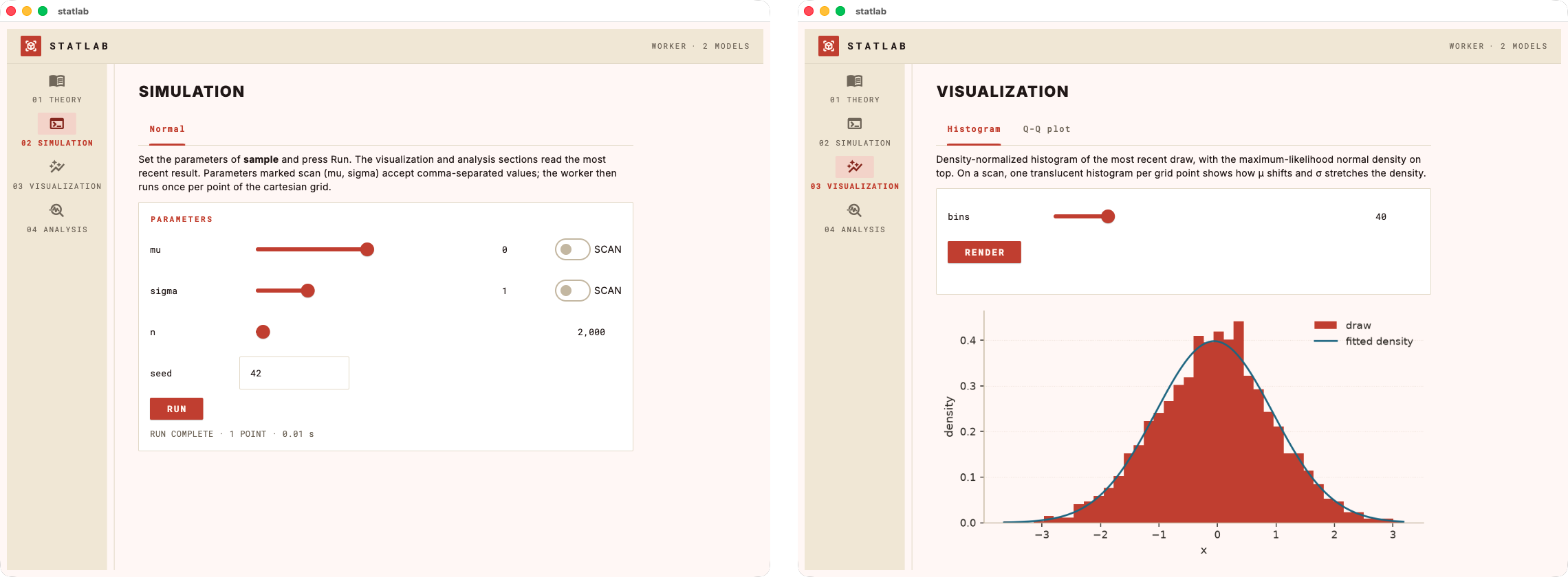
Quick start
import matplotlib.pyplot as plt
import numpy as np

import labforge
from labforge import Lab, Param, ScanResult

lab = Lab("gausslab")
lab.set_theory("theory.md")   # markdown file or string; $$...$$ becomes LaTeX


def sample(mu=0.0, sigma=1.0, n=2000, seed=42):
    """Draw n Gaussian variates; reproducible for a given seed."""
    return np.random.default_rng(seed).normal(mu, sigma, n)


lab.add_worker(sample, {
    "mu": Param(default=0.0, bounds=(-5, 5), scan=True),
    "sigma": Param(default=1.0, bounds=(0.1, 4), scan=True),
    "n": Param(kind="int", default=2000, bounds=(10, 100_000)),
    "seed": "int",
})


def histogram(data, bins=40):
    fig, ax = plt.subplots(figsize=(7, 3.4))
    if isinstance(data, ScanResult):   # a parameter scan: one histogram per grid point
        for params, draws in data:
            ax.hist(draws, bins=bins, density=True, alpha=0.5,
                    label=", ".join(f"{k} = {params[k]:g}" for k in data.keys))
        ax.legend()
    else:
        ax.hist(data, bins=bins, density=True, color=labforge.palette().data)
    labforge.style(fig, ax)            # optional house treatment
    return fig, ax


lab.add_viz(histogram, "Histogram", "Density histogram of the draw.",
            {"bins": Param(kind="int", default=40, bounds=(5, 200))})


def moments(data):
    if isinstance(data, ScanResult):   # one table row per grid point
        return [{**params, "mean": float(np.mean(d)), "std": float(np.std(d))}
                for params, d in data]
    return {"mean": float(np.mean(data)), "std": float(np.std(data, ddof=1))}


lab.add_analysis(moments, "Moments", "Sample moments of the draw.")

lab.open()
That is the whole app. lab.open() opens a native window with four pages —
Theory, Simulation, Visualization, Analysis — a slider for every bounded
parameter, a Run button, and tabs for each registered visualization and
analysis.
An extended version of this example — same lab plus a fitted-density overlay
and a Q-Q plot tab — lives at examples/demo_lab.py:
python examples/demo_lab.py                 # native window
python examples/demo_lab.py --browser 8550  # serve at http://localhost:8550
python examples/demo_lab.py --scroll        # one continuous scrolling page
python examples/demo_lab.py --theme lavender
Concepts
Worker. One function produces the data. Each keyword argument gets a UI
control from its Param spec — or from the signature default alone, if you
spec nothing:
| spec | control |
|---|---|
Param(default=1.0, bounds=(0, 5)) |
slider with live readout |
Param(kind="int", default=100, bounds=(10, 1000)) |
integer slider |
Param(default=1.0) / "scalar" / "int" |
validated text field |
Param(..., scan=True) / "scalar or array" / "int or array" |
scannable (see below) |
"N-tuple" (e.g. "2-tuple") |
one field per element |
Validation happens at registration: unknown spec keys, defaults outside
bounds, or a scan spec on a non-worker function raise ValueError when the
app is assembled, never mid-use.
Parameter scans. A kwarg declared scan=True gets a scan toggle (bounded)
or a comma-separated field (unbounded). Enter 0, 1, 2 and labforge calls the
worker once per point of the cartesian grid across all scanned parameters —
the worker itself always receives scalars. Downstream functions then receive a
ScanResult: a list of (params, result) records with keys, values() and
axis(name) helpers, distinguished with isinstance(data, ScanResult).
Visualizations. Functions viz(data, **kwargs) returning a matplotlib
figure (bare or (fig, ax)). Each gets a tab with its own controls and a
Render button. Figures are yours — labforge only serializes them; the house
style (labforge.style(fig, ax)) is strictly opt-in.
Analyses. Functions analysis(data, **kwargs) — the return shape picks
the rendering:
| return | rendered as |
|---|---|
dict |
two-column quantity/value table |
list of dicts, or a DataFrame |
full table |
str |
markdown |
Figure or (fig, ax) |
image |
| anything else | its repr |
Multiple workers. Call add_worker more than once for a lab with several
workers. Each worker keeps its own workspace — its controls, its last result and
its per-tab settings — and the add_viz / add_analysis calls after each
add_worker attach that worker's own tabs, so switching workers and back
restores exactly what was there. Several workers need a way to choose among them
(checked at build): a selects_worker model selector, or worker_view="tabs"
to lay the workers out as Simulation-page tabs.
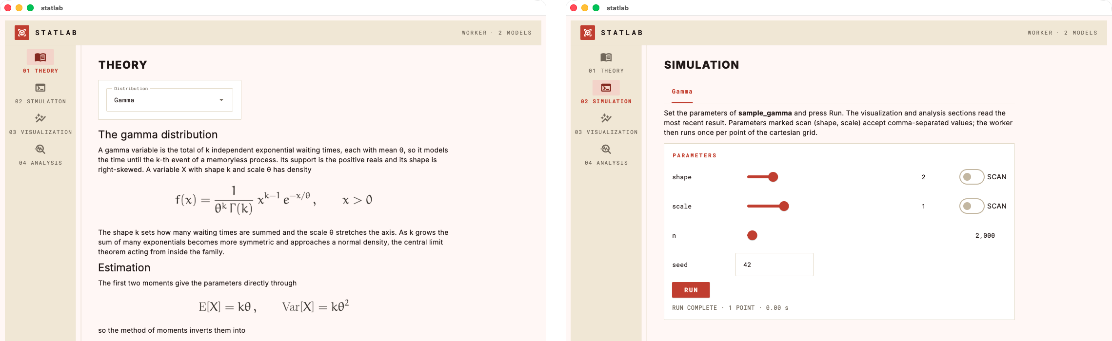
The clean way is a Theory-page selector with selects_worker=True: its options
name the workers, so choosing one both swaps the theory and makes that worker
active. There is no top-bar dropdown; the Simulation page shows the active
worker as a single tab, matching the tabbed Visualization and Analysis pages.
The demo (examples/demo_lab.py) uses this to switch between a normal and a
gamma model:
lab.set_theory_selector(
    "model",
    Param(kind="choice", options=["Normal", "Gamma"]),
    theory_for,                 # theory_for(selection) -> markdown
    label="Distribution",
    selects_worker=True,
)
lab.add_worker(sample, {...}, name="Normal")   # its own viz/analysis tabs
lab.add_worker(sample_gamma, {...}, name="Gamma")
Theory. A markdown file or string. Displayed $$...$$ equations render as
crisp images — through your system LaTeX toolchain when one is installed
(with the Euler math font), falling back to matplotlib's mathtext otherwise.
Layouts, views and themes
lab.open() takes four independent knobs:
view="app"(native window, default) or"browser"— serve the same app and open it in your web browser; with a fixedportthe URL is stable across relaunches, and every browser tab gets its own isolated session.layout="pages"(rail navigation, default) or"scroll"— the whole lab as one continuous scrolling page.theme— one of eight palettes, four dark and four light. A theme sets the chrome, the plot palette and the equation ink together, so figures never drift from the app around them. Colour your own figures withlabforge.palette().data,.model,.highlight; list the options withlabforge.themes():
| name | mode | look |
|---|---|---|
paper |
light | warm paper surfaces, graphite ink, vermilion accent (default) |
mint |
light | light mint greens on white |
glacier |
light | pale glacier blues, deep slate accent |
lavender |
light | soft lavender neutrals, deep violet accent |
retro_green |
dark | matrix mood, calmer green, legible olive card |
instrument |
dark | near-black teal-tinted surfaces, one electric accent |
neon_violet |
dark | violet chrome, hot-pink data |
neon_gold |
dark | the violet palette with pale gold as the accent |
The Theory page under each theme — the equations are real LaTeX, rendered in the theme's ink:
paper 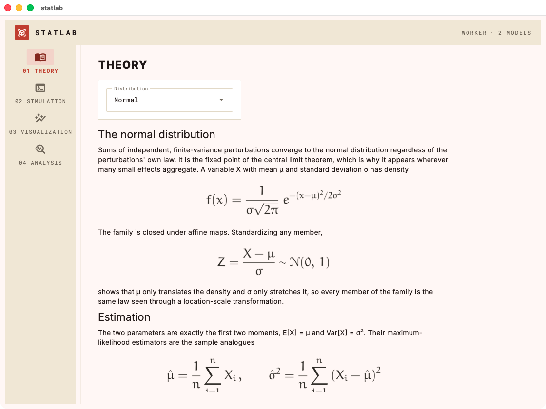 |
mint 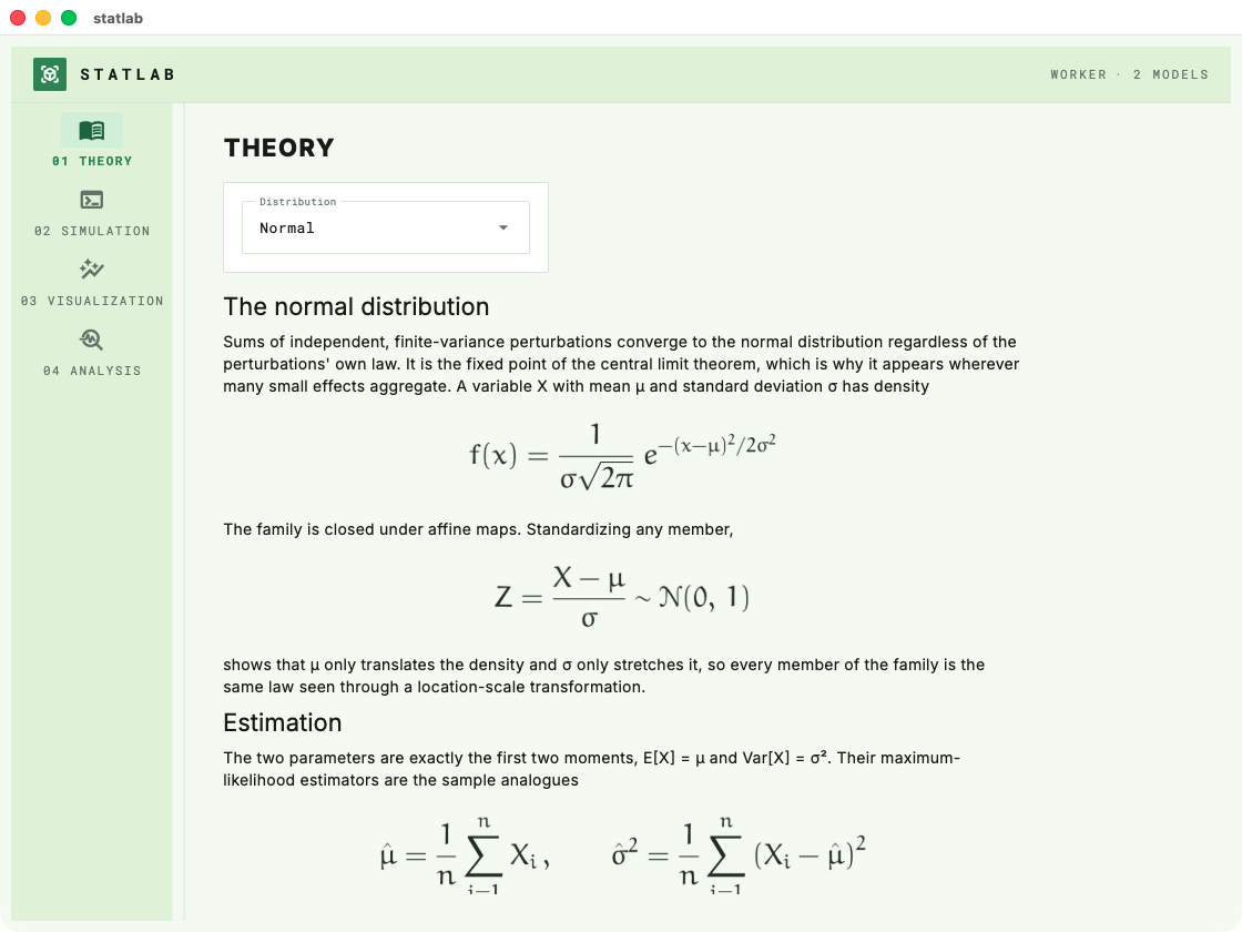 |
glacier 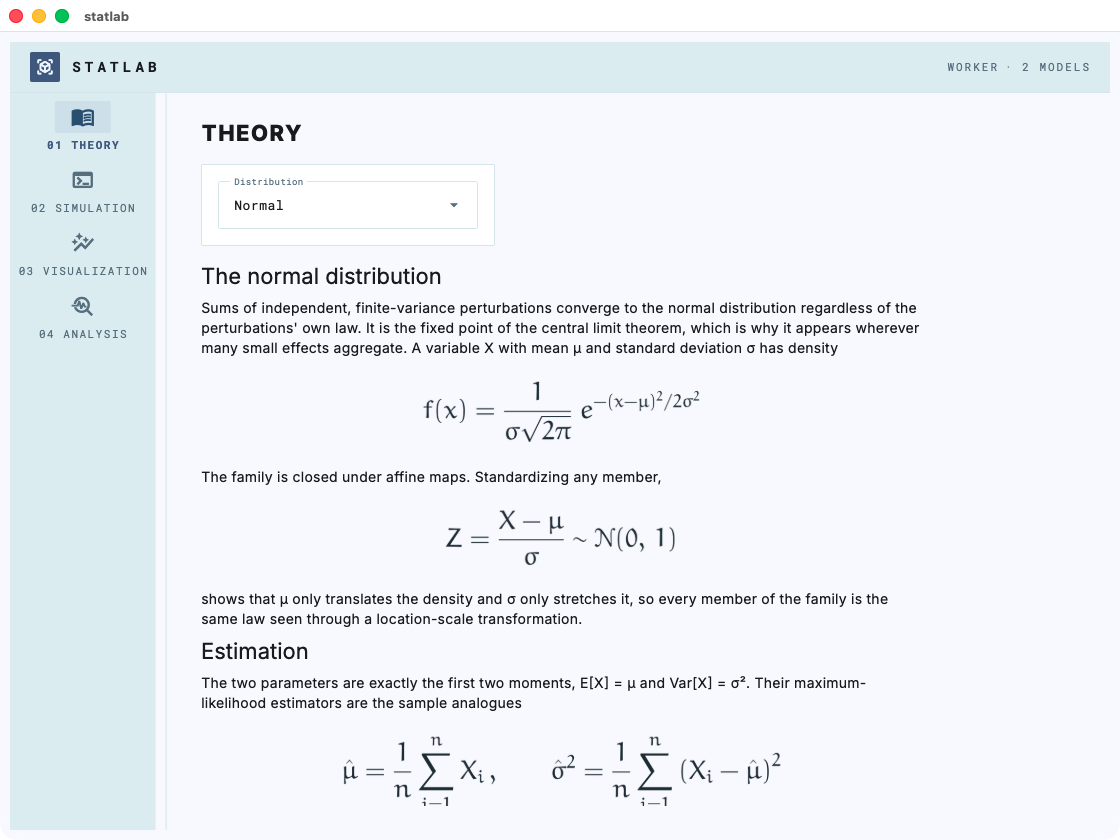 |
lavender 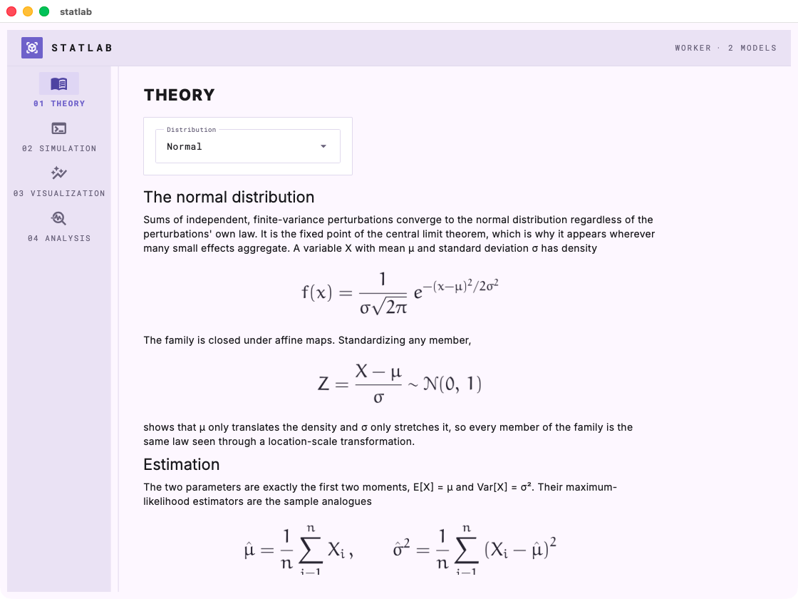 |
retro_green 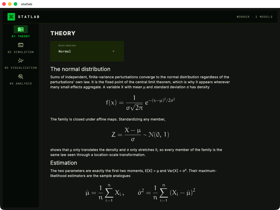 |
instrument 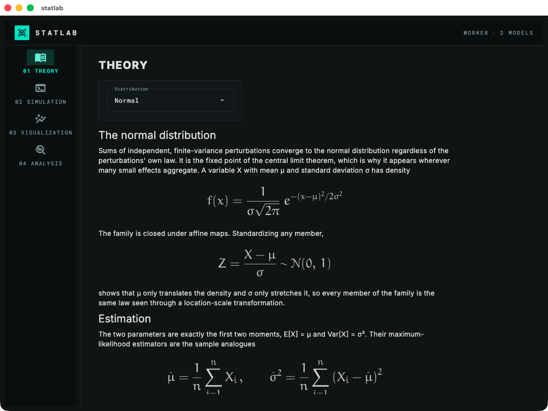 |
neon_violet 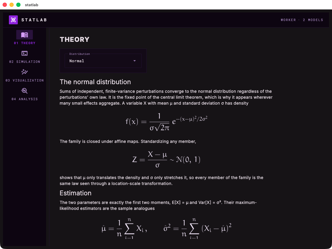 |
neon_gold 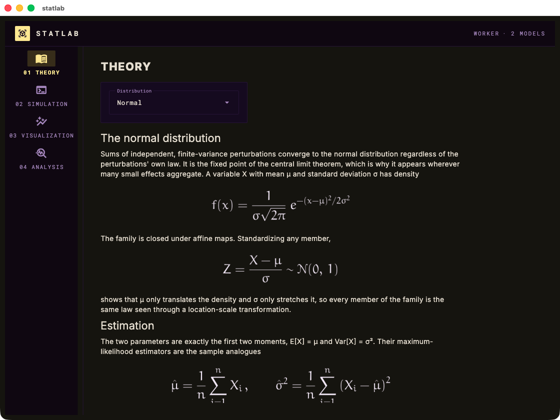 |
Install
Requires Python ≥ 3.10.
pip install labforge
Or from a clone, if you want to work on the code directly:
git clone https://github.com/laroccod/labforge.git
cd labforge
pip install -e .
Dependencies: flet (pinned), numpy, matplotlib. A system LaTeX
toolchain (latex + dvipng) is optional and only affects equation
typography.
Development
pip install -e ".[dev]"
pytest                                        # unit + offline page-tree smoke tests
black --check --line-length 100 src tests examples
The test suite builds every page and layout headlessly — no window needed — and asserts that equations and figures actually rendered, so most mistakes are caught without launching the app.
License


Download files
Download the file for your platform. If you're not sure which to choose, learn more about installing packages.
Source Distribution
Built Distribution
Filter files by name, interpreter, ABI, and platform.
If you're not sure about the file name format, learn more about wheel file names.
Copy a direct link to the current filters
File details
Details for the file labforge-0.2.0.tar.gz.
File metadata
- Download URL: labforge-0.2.0.tar.gz
- Upload date:
- Size: 2.0 MB
- Tags: Source
- Uploaded using Trusted Publishing? No
- Uploaded via: twine/6.2.0 CPython/3.13.13
File hashes
| Algorithm | Hash digest | |
|---|---|---|
| SHA256 |
ae18c81aa3aaf91b93a7b547c4a262f6aa3339f95c368adf3c3e15a5d78c5041
|
|
| MD5 |
bd30a0c30d9245707ff103050bd3ead9
|
|
| BLAKE2b-256 |
68174ea38f24d398a44c29c40f59eb98994c24aced0ec22992773e3f62377d9c
|
File details
Details for the file labforge-0.2.0-py3-none-any.whl.
File metadata
- Download URL: labforge-0.2.0-py3-none-any.whl
- Upload date:
- Size: 635.7 kB
- Tags: Python 3
- Uploaded using Trusted Publishing? No
- Uploaded via: twine/6.2.0 CPython/3.13.13
File hashes
| Algorithm | Hash digest | |
|---|---|---|
| SHA256 |
58b0481637c24645138287ef113fc56aa5edabb46e6ebd034f2599816229ef55
|
|
| MD5 |
13b337c09b93085d485f092afc0e56f9
|
|
| BLAKE2b-256 |
1cf9abd107dcf58a1bef4e63390f7c105d179e45db6f1f3c7e7554e47ab53e1f
|






