A reader for Canadian Well Logging Society LAS (Log ASCII Standard) files.
Project description
The las module implements a reader for LAS (Log ASCII Standard) well log files (LAS 2.0). For more information about this format, see the Canadian Well Logging Society web page (https://www.cwls.org/products/).
Example 1
The following file, “example1.las”, is from “LAS Version 2.0: A Digital Standard for Logs; Updated January 2014”:
~VERSION INFORMATION
VERS.                          2.0 :   CWLS LOG ASCII STANDARD -VERSION 2.0
WRAP.                          NO  :   ONE LINE PER DEPTH STEP
~WELL INFORMATION
#MNEM.UNIT              DATA                       DESCRIPTION
#----- -----            ----------               -------------------------
STRT    .M              1670.0000                :START DEPTH
STOP    .M              1669.7500                :STOP DEPTH
STEP    .M              -0.1250                  :STEP
NULL    .               -999.25                  :NULL VALUE
COMP    .       ANY OIL COMPANY INC.             :COMPANY
WELL    .       ANY ET AL 12-34-12-34            :WELL
FLD     .       WILDCAT                          :FIELD
LOC     .       12-34-12-34W5M                   :LOCATION
PROV    .       ALBERTA                          :PROVINCE
SRVC    .       ANY LOGGING COMPANY INC.         :SERVICE COMPANY
DATE    .       13-DEC-86                        :LOG DATE
UWI     .       100123401234W500                 :UNIQUE WELL ID
~CURVE INFORMATION
#MNEM.UNIT              API CODES                   CURVE DESCRIPTION
#------------------     ------------              -------------------------
 DEPT   .M                                       :  1  DEPTH
 DT     .US/M           60 520 32 00             :  2  SONIC TRANSIT TIME
 RHOB   .K/M3           45 350 01 00             :  3  BULK DENSITY
 NPHI   .V/V            42 890 00 00             :  4  NEUTRON POROSITY
 SFLU   .OHMM           07 220 04 00             :  5  SHALLOW RESISTIVITY
 SFLA   .OHMM           07 222 01 00             :  6  SHALLOW RESISTIVITY
 ILM    .OHMM           07 120 44 00             :  7  MEDIUM RESISTIVITY
 ILD    .OHMM           07 120 46 00             :  8  DEEP RESISTIVITY
~PARAMETER INFORMATION
#MNEM.UNIT              VALUE             DESCRIPTION
#--------------     ----------------      -----------------------------------------------
 MUD    .               GEL CHEM        :   MUD TYPE
 BHT    .DEGC           35.5000         :   BOTTOM HOLE TEMPERATURE
 BS     .MM             200.0000        :   BIT SIZE
 FD     .K/M3           1000.0000       :   FLUID DENSITY
 MATR   .               SAND            :   NEUTRON MATRIX
 MDEN   .               2710.0000       :   LOGGING MATRIX DENSITY
 RMF    .OHMM           0.2160          :   MUD FILTRATE RESISTIVITY
 DFD    .K/M3           1525.0000       :   DRILL FLUID DENSITY
~OTHER
     Note: The logging tools became stuck at 625 metres causing the data
     between 625 metres and 615 metres to be invalid.
~A  DEPTH     DT    RHOB        NPHI   SFLU    SFLA      ILM      ILD
1670.000   123.450 2550.000    0.450  123.450  123.450  110.200  105.600
1669.875   123.450 2550.000    0.450  123.450  123.450  110.200  105.600
1669.750   123.450 2550.000    0.450  123.450  123.450  110.200  105.600
Sample python session:
>>> import las
>>> log = las.LASReader('example1.las')
>>> log.start
1670.0
>>> log.stop
1669.75
>>> log.step
-0.125
>>> log.null
-999.25
>>> log.well.COMP
LASItem(name='COMP', units='', data='ANY OIL COMPANY INC.', descr='COMPANY')
>>> log.well.COMP.value
'ANY OIL COMPANY INC.'
>>> log.well.FLD.value
'WILDCAT'
>>> print(log.other)
     Note: The logging tools became stuck at 625 metres causing the data
     between 625 metres and 615 metres to be invalid.
The log data is stored as a numpy structured array in log.data:
>>> log.data
array([(1670.0, 123.45, 2550.0, 0.45, 123.45, 123.45, 110.2, 105.6),
       (1669.875, 123.45, 2550.0, 0.45, 123.45, 123.45, 110.2, 105.6),
       (1669.75, 123.45, 2550.0, 0.45, 123.45, 123.45, 110.2, 105.6)],
      dtype=[('DEPT', '<f8'), ('DT', '<f8'), ('RHOB', '<f8'), ('NPHI', '<f8'), ('SFLU', '<f8'), ('SFLA', '<f8'), ('ILM', '<f8'), ('ILD', '<f8')])
>>> log.data['RHOB']
array([ 2550.,  2550.,  2550.])
>>> log.data[0]
(1670.0, 123.45, 2550.0, 0.45, 123.45, 123.45, 110.2, 105.6)
The data is also available as a two-dimensional numpy array. First we’ll adjust numpy’s output format. This is not necessary, but it makes the values easier to read:
>>> import numpy as np
>>> np.set_printoptions(precision=4)
The two-dimensional view of the data is called data2d:
>>> log.data2d
array([[  1.6700e+03,   1.2345e+02,   2.5500e+03,   4.5000e-01,
          1.2345e+02,   1.2345e+02,   1.1020e+02,   1.0560e+02],
       [  1.6699e+03,   1.2345e+02,   2.5500e+03,   4.5000e-01,
          1.2345e+02,   1.2345e+02,   1.1020e+02,   1.0560e+02],
       [  1.6698e+03,   1.2345e+02,   2.5500e+03,   4.5000e-01,
          1.2345e+02,   1.2345e+02,   1.1020e+02,   1.0560e+02]])
>>> log.data2d.shape
(3, 8)
Example 2
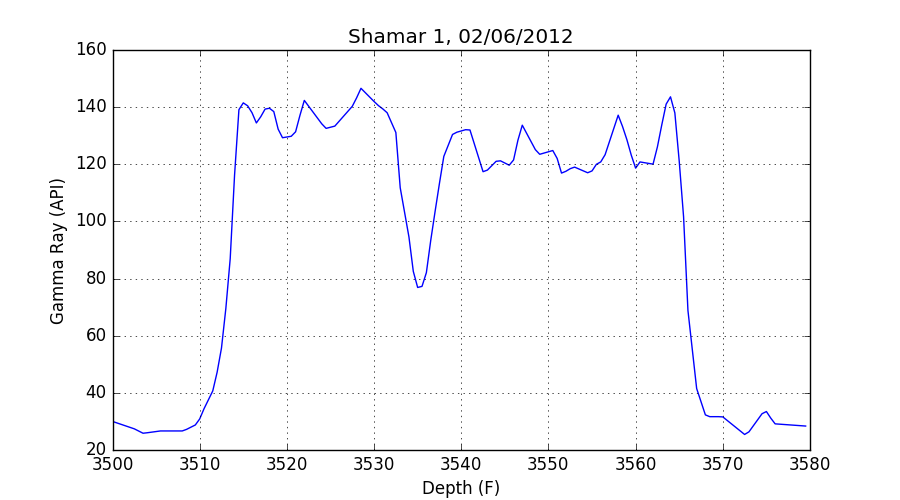
The next example reads a file from the Kansas Geological Survey and makes a plot of the gamma ray data versus depth using matplotlib.
First, the imports:
>>> import numpy as np
>>> import matplotlib.pyplot as plt
>>> import las
>>> import io
>>> try:
...     from urllib.request import urlopen
... except ImportError:
...     from urllib import urlopen
...
Next, read the file:
>>> url = "http://www.kgs.ku.edu/software/DEWL/HELP/pc_read/Shamar-1.las"
>>> f = io.StringIO(urlopen(url).read().decode('iso-8859-1'))
>>> log = las.LASReader(f, null_subs=np.nan)
Finally, make the plot using matplotlib:
>>> plt.figure(figsize=(9, 5))
>>> plt.plot(log.data['DEPT'], log.data['GR'])
>>> plt.xlabel(log.curves.DEPT.descr + " (%s)" % log.curves.DEPT.units)
>>> plt.ylabel(log.curves.GR.descr + " (%s)" % log.curves.GR.units)
>>> plt.title(log.well.WELL.data + ', ' + log.well.DATE.data)
>>> plt.grid()
>>> plt.show()

Project details
Download files
Download the file for your platform. If you're not sure which to choose, learn more about installing packages.
Source Distribution
Built Distribution
Filter files by name, interpreter, ABI, and platform.
If you're not sure about the file name format, learn more about wheel file names.
Copy a direct link to the current filters
File details
Details for the file las-0.0.5.tar.gz.
File metadata
- Download URL: las-0.0.5.tar.gz
- Upload date:
- Size: 10.6 kB
- Tags: Source
- Uploaded using Trusted Publishing? No
- Uploaded via: twine/5.0.0 CPython/3.12.3
File hashes
| Algorithm | Hash digest | |
|---|---|---|
| SHA256 |
3e867fa5e8b4e7ffb08c4a8a92636b04cf16cfbc7e5d97b9f0420d9d8e4171e1
|
|
| MD5 |
6617c24ec7a1eece6380cb49005ab685
|
|
| BLAKE2b-256 |
7be30b7273a0953707d8004075c5f74a31aa53eb02f943f00e25f935b26fbc51
|
File details
Details for the file las-0.0.5-py3-none-any.whl.
File metadata
- Download URL: las-0.0.5-py3-none-any.whl
- Upload date:
- Size: 8.0 kB
- Tags: Python 3
- Uploaded using Trusted Publishing? No
- Uploaded via: twine/5.0.0 CPython/3.12.3
File hashes
| Algorithm | Hash digest | |
|---|---|---|
| SHA256 |
a7226635e63f66003a8d244e0523f77f4901860dc9c2869de420cd987aae62f9
|
|
| MD5 |
4ae8444c317c255f6d7d2e663cfb2c74
|
|
| BLAKE2b-256 |
72d72f21b9fda3d6abe0bdfe5b5ea29e968ed6b9157690b11eae23740129b5bd
|


