Simple and efficient Python package for modeling d-dimensional Bravais lattices in solid state physics.

Project description
LattPy - Simple Lattice Modeling in Python


:warning: WARNING: This project is still in development and might change significantly in the future!
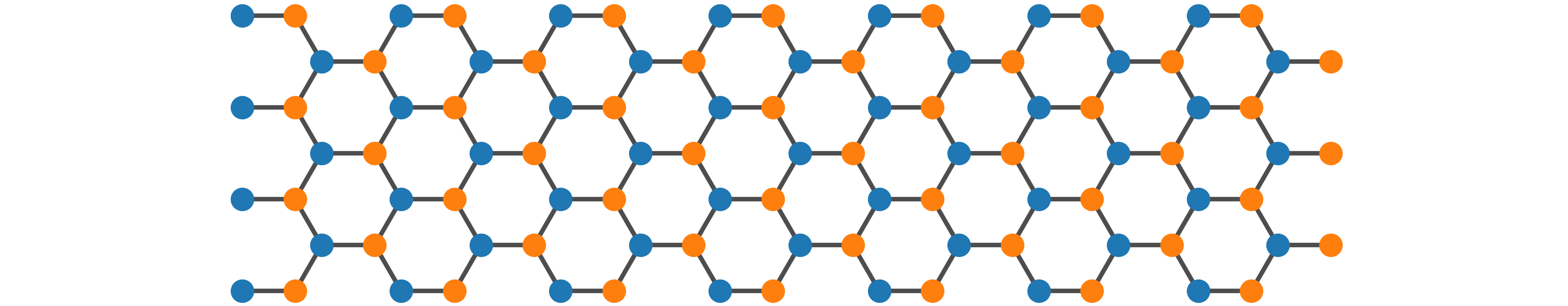
LattPy is a simple and efficient Python package for modeling Bravais lattices and constructing (finite) lattice structures in any dimension. It provides an easy interface for constructing lattice structures by simplifying the configuration of the unit cell and the neighbor connections - making it possible to construct complex models in just a few lines of code and without the headache of adding neighbor connections manually. You will save time and mental energy for more important matters.
| Master |  |
 |
 |
|---|---|---|---|
| Dev |  |
 |
 |
🔧 Installation
LattPy is available on PyPI:
pip install lattpy
Alternatively, it can be installed via GitHub
pip install git+https://github.com/dylanljones/lattpy.git@VERSION
where VERSION is a release or tag. The project can also be
cloned/forked and installed via
python setup.py install
📖 Documentation
Read the documentation on ReadTheDocs!
🚀 Quick-Start
See the tutorial for more information and examples.
Features:
- Basis transformations
- Configurable unit cell
- Easy neighbor configuration
- General lattice structures
- Finite lattice models in world or lattice coordinates
- Periodic boundary conditions along any axis
Configuration
A new instance of a lattice model is initialized using the unit-vectors of the Bravais lattice.
After the initialization the atoms of the unit-cell need to be added. To finish the configuration
the connections between the atoms in the lattice have to be set. This can either be done for
each atom-pair individually by calling add_connection or for all possible pairs at once by
callling add_connections. The argument is the number of unique
distances of neighbors. Setting a value of 1 will compute only the nearest
neighbors of the atom.
import numpy as np
from lattpy import Lattice

latt = Lattice(np.eye(2))                 # Construct a Bravais lattice with square unit-vectors
latt.add_atom(pos=[0.0, 0.0])             # Add an Atom to the unit cell of the lattice
latt.add_connections(1)                   # Set the maximum number of distances between all atoms

latt = Lattice(np.eye(2))                 # Construct a Bravais lattice with square unit-vectors
latt.add_atom(pos=[0.0, 0.0], atom="A")   # Add an Atom to the unit cell of the lattice
latt.add_atom(pos=[0.5, 0.5], atom="B")   # Add an Atom to the unit cell of the lattice
latt.add_connection("A", "A", 1)          # Set the max number of distances between A and A
latt.add_connection("A", "B", 1)          # Set the max number of distances between A and B
latt.add_connection("B", "B", 1)          # Set the max number of distances between B and B
latt.analyze()
Configuring all connections using the add_connections-method will call the analyze-method
directly. Otherwise this has to be called at the end of the lattice setup or by using
analyze=True in the last call of add_connection. This will compute the number of neighbors,
their distances and their positions for each atom in the unitcell.
To speed up the configuration prefabs of common lattices are included. The previous lattice can also be created with
from lattpy import simple_square

latt = simple_square(a=1.0, neighbors=1)  # Initializes a square lattice with one atom in the unit-cell
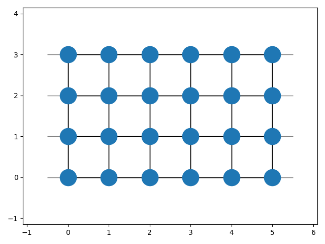
So far only the lattice structure has been configured. To actually construct a (finite) model of the lattice the model has to be built:
latt.build(shape=(5, 3))
This will compute the indices and neighbors of all sites in the given shape and store the data.
After building the lattice periodic boundary conditions can be set along one or multiple axes:
latt.set_periodic(axis=0)
To view the built lattice the plot-method can be used:
import matplotlib.pyplot as plt

latt.plot()
plt.show()
General lattice attributes
After configuring the lattice the attributes are available.
Even without building a (finite) lattice structure all attributes can be computed on the fly for a given lattice vector,
consisting of the translation vector n and the atom index alpha. For computing the (translated) atom positions
the get_position method is used. Also, the neighbors and the vectors to these neighbors can be calculated.
The dist_idx-parameter specifies the distance of the neighbors (0 for nearest neighbors, 1 for next nearest neighbors, ...):
from lattpy import simple_square

latt = simple_square()

# Get position of atom alpha=0 in the translated unit-cell
positions = latt.get_position(n=[0, 0], alpha=0)

# Get lattice-indices of the nearest neighbors of atom alpha=0 in the translated unit-cell
neighbor_indices = latt.get_neighbors(n=[0, 0], alpha=0, distidx=0)

# Get vectors to the nearest neighbors of atom alpha=0 in the translated unit-cell
neighbor_vectors = latt.get_neighbor_vectors(alpha=0, distidx=0)
Also, the reciprocal lattice vectors can be computed
rvecs = latt.reciprocal_vectors()
or used to construct the reciprocal lattice:
rlatt = latt.reciprocal_lattice()
The 1. Brillouin zone is the Wigner-Seitz cell of the reciprocal lattice:
bz = rlatt.wigner_seitz_cell()
The 1.BZ can also be obtained by calling the explicit method of the direct lattice:
bz = latt.brillouin_zone()
Finite lattice data
If the lattice has been built the needed data is cached. The lattice sites of the
structure then can be accessed by a simple index i. The syntax is the same as before,
just without the get_ prefix:
latt.build((5, 2))
i = 2

# Get position of the atom with index i=2
positions = latt.position(i)

# Get the atom indices of the nearest neighbors of the atom with index i=2
neighbor_indices = latt.neighbors(i, distidx=0)

# the nearest neighbors can also be found by calling (equivalent to dist_idx=0)
neighbor_indices = latt.nearest_neighbors(i)
Data map
The lattice model makes it is easy to construct the (tight-binding) Hamiltonian of a non-interacting model:
import numpy as np
from lattpy import simple_chain

# Initializes a 1D lattice chain with a length of 5 atoms.
latt = simple_chain(a=1.0)
latt.build(shape=4)
n = latt.num_sites

# Construct the non-interacting (kinetic) Hamiltonian-matrix
eps, t = 0., 1.
ham = np.zeros((n, n))
for i in range(n):
    ham[i, i] = eps
    for j in latt.nearest_neighbors(i):
        ham[i, j] = t
Since we loop over all sites of the lattice the construction of the hamiltonian is slow.
An alternative way of mapping the lattice data to the hamiltonian is using the DataMap
object returned by the map() method of the lattice data. This stores the atom-types,
neighbor-pairs and corresponding distances of the lattice sites. Using the built-in
masks the construction of the hamiltonian-data can be vectorized:
from scipy import sparse

# Vectorized construction of the hamiltonian
eps, t = 0., 1.
dmap = latt.data.map()               # Build datamap
values = np.zeros(dmap.size)         # Initialize array for data of H
values[dmap.onsite(alpha=0)] = eps   # Map onsite-energies to array
values[dmap.hopping(distidx=0)] = t  # Map hopping-energies to array

# The indices and data array can be used to construct a sparse matrix
ham_s = sparse.csr_matrix((values, dmap.indices))
ham = ham_s.toarray()
Both construction methods will create the following Hamiltonian-matrix:
[[0. 1. 0. 0. 0.]
 [1. 0. 1. 0. 0.]
 [0. 1. 0. 1. 0.]
 [0. 0. 1. 0. 1.]
 [0. 0. 0. 1. 0.]]
🔥 Performance
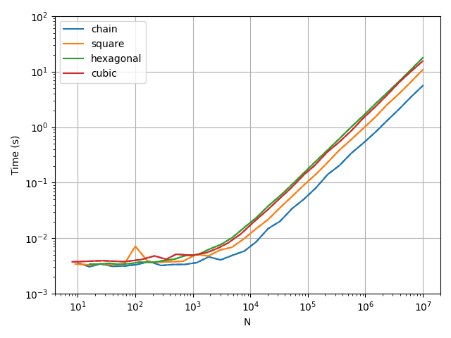
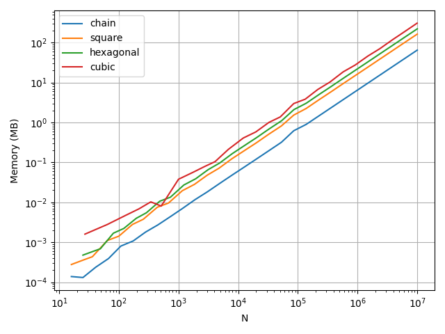
Even though lattpy is written in pure python, it achieves high performance and
a low memory footprint by making heavy use of numpy's vectorized operations and scipy's
cKDTree. As an example the build times and memory usage in the build process for different
lattices are shown in the following plots:
| Build time | Build memory |
|---|---|
 |
 |
Note that the overhead of the multi-thread neighbor search results in a slight
increase of the build time for small systems. By using num_jobs=1 in the build-method
this overhead can be eliminated for small systems. By passing num_jobs=-1 all cores
of the system are used.
💻 Development
See the CHANGELOG for the recent changes of the project.
If you encounter an issue or want to contribute to pyrekordbox, please feel free to
get in touch, create an issue
or open a pull request! A guide for contributing to lattpy and the commit-message style can be found in
CONTRIBUTING
Release history Release notifications | RSS feed


Download files
Download the file for your platform. If you're not sure which to choose, learn more about installing packages.
Source Distribution
Built Distribution
Filter files by name, interpreter, ABI, and platform.
If you're not sure about the file name format, learn more about wheel file names.
Copy a direct link to the current filters
File details
Details for the file lattpy-0.7.7.tar.gz.
File metadata
- Download URL: lattpy-0.7.7.tar.gz
- Upload date:
- Size: 309.3 kB
- Tags: Source
- Uploaded using Trusted Publishing? No
- Uploaded via: twine/4.0.1 CPython/3.9.15
File hashes
| Algorithm | Hash digest | |
|---|---|---|
| SHA256 |
c69c56a777955ad0b54a98f61c0f4e95266981b6320e6b0be3b08bc0265c4b8d
|
|
| MD5 |
071fbfa459a4ea58ad3b85651e10e7a6
|
|
| BLAKE2b-256 |
4e50f1596a8114b546365699498d6cc2df74b5deb14f0932095a6a0b81eec068
|
File details
Details for the file lattpy-0.7.7-py3-none-any.whl.
File metadata
- Download URL: lattpy-0.7.7-py3-none-any.whl
- Upload date:
- Size: 79.2 kB
- Tags: Python 3
- Uploaded using Trusted Publishing? No
- Uploaded via: twine/4.0.1 CPython/3.9.15
File hashes
| Algorithm | Hash digest | |
|---|---|---|
| SHA256 |
d488e9ede646f15f3520308d9c0afeb606fb6a36b6e3f7677919e42f58a2ef72
|
|
| MD5 |
9d4d57e69eefeac8b4aa978827c67608
|
|
| BLAKE2b-256 |
ec186234067786abc676fafc6519d3c820aa1fb5e64c5b509794a61f20115001
|


