Simple Python tools for plotting learning curves of neural network models trained with the Keras, Ultralytics YOLO or scikit-learn framework in a single figure in an easy-to-understand format.

Project description
LCurveTools
Simple Python tools for plotting learning curves of neural network models trained with the Keras, Ultralytics YOLO or scikit-learn framework in a single figure in an easy-to-understand format.
Currently the lcurvetools package provides three basic functions: lcurves, history_concatenate and lcurves_by_MLP_estimator.
NOTE: All of the plotting examples below are for interactive Python mode in Jupyter-like environments. If you are in non-interactive mode you may need to explicitly call plt.show() after calling the lcurves or lcurves_by_MLP_estimator function to display the window with built plots on your screen.
Installation
The easiest way to install the lcurvetools package for the first time is using pip:
pip install lcurvetools
To update a previously installed package to the latest version, use the command:
pip install lcurvetools --upgrade
The lcurves function to plot learning curves based on model training history dictionaries
The lcurves function and its alias lcurves_by_history plot learning curves based on a dictionary or a list of dictionaries with model training histories. Each dictionary with a history should contain keys with training and validation values of losses and metrics, as well as learning rate values at successive epochs, for example:
{"loss": [0.5, 0.3, 0.2], "val_loss": [0.6, 0.4, 0.25], "accuracy": [0.7, 0.8, 0.85], "val_accuracy": [0.65, 0.75, 0.8], "lr": [0.01, 0.01, 0.001]}. This training history format is adopted in the Keras library and is also widely used when working with other libraries.
Neural network model training with Keras is performed using the fit method. The method returns the History object with the history attribute which is dictionary and contains keys with training and validation values of losses and metrics, as well as learning rate values at successive epochs. The lcurves function and its alias lcurves_by_history use the History.history dictionary to plot the learning curves as the dependences of the above values on the epoch index.
Import the keras module and the lcurves function:
import keras
from lcurvetools import lcurves
Plotting learning curves of one model based on one dictionary
Usage scheme
-
Create, compile and fit the keras model:
model = keras.Model(...) # or keras.Sequential(...)
model.compile(...)
hist = model.fit(...)
-
Use
hist.historydictionary to plot the learning curves as the dependences of values of all keys in the dictionary on an epoch index with automatic recognition of keys of losses, metrics and learning rate:lcurves(hist.history);
Typical appearance of the output figure
The appearance of the output figure depends on the list of keys in the hist.history dictionary, which is determined by the parameters of the compile and fit methods of the model. For example, for a typical usage of these methods, the list of keys would be ['loss', 'accuracy', 'val_loss', 'val_accuracy'] and the output figure will contain 2 subplots with loss and metrics vertical axes and might look like this:
model.compile(loss="categorical_crossentropy", metrics=["accuracy"])
hist = model.fit(x_train, y_train, validation_split=0.1, epochs=50)
lcurves(hist.history);
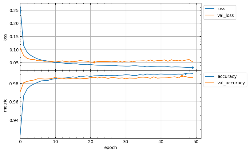
Of course, if the metrics parameter of the compile method is not specified, then the output figure will not contain a metric subplot.
Minimum values of loss curves and the best values of metric curves are marked by points. The best values of metrics are determined based on the specified optimization mode for each metric (see optimization_modes parameter). By default, the optimization modes are determined automatically based on metric name with the lcurves.utils.get_mode_by_metric_name function.
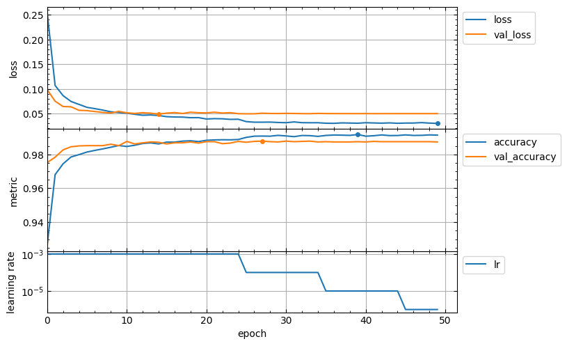
Usage of callbacks for the fit method can add new keys to the hist.history dictionary. For example, the ReduceLROnPlateau callback adds the lr key with learning rate values for successive epochs. In this case the output figure will contain additional subplot with learning rate vertical axis in a logarithmic scale and might look like this:
hist = model.fit(x_train, y_train, validation_split=0.1, epochs=50,
    callbacks=[keras.callbacks.ReduceLROnPlateau()],
)
lcurves(hist.history);
Customizing appearance of the output figure
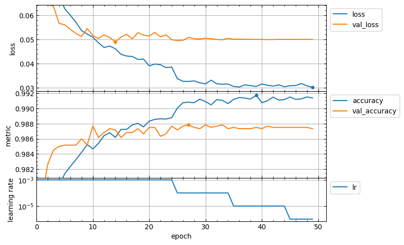
The lcurves function has optional parameters to customize the appearance of the output figure. For example, the epoch_range_to_scale option allows to specify the epoch index range within which the subplots of the losses and metrics are scaled.
- If
epoch_range_to_scaleis a list or a tuple of two int values, then they specify the epoch index limits of the scaling range in the form[start, stop), i.e. as forsliceandrangeobjects. - If
epoch_range_to_scaleis an int value, then it specifies the lower epoch indexstartof the scaling range, and the losses and metrics subplots are scaled by epochs with indices fromstartto the last.
So, you can exclude the first 5 epochs from the scaling range as follows:
lcurves(hist.history, epoch_range_to_scale=5);
For a description of other optional parameters of the lcurves function to customize the appearance of the output figure, see its docstring.
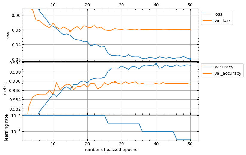
The lcurves function returns a numpy array or a list of the matplotlib.axes.Axes objects corresponded to the built subplots from top to bottom. So, you can use the methods of these objects to customize the appearance of the output figure.
axs = lcurves(history, epoch_range_to_scale=6)
axs[0].tick_params(axis="x", labeltop=True)
axs[-1].set_xlabel('number of passed epochs')
axs[-1].legend().remove()
Plotting learning curves based on a list of dictionaries with fitting histories of several models
Usage scheme
-
Create, compile and fit the several keras models:
model_1 = keras.Model(...) # or keras.Sequential(...)
model_1.compile(...)
hist_1 = model.fit(...)

model_2 = keras.Model(...) # or keras.Sequential(...)
model_2.compile(...)
hist_2 = model.fit(...)

<...>
-
Use a list of dictionaries
[hist_1.history, hist_2.history, ...]to plot all learning curves of all models in a single figure:lcurves([hist_1.history, hist_2.history, ...]);
Plotting learning curves based on a list of dictionaries with independent refitting histories of one model
Usage scheme
-
Organize a loop of multiple independent retraining of the model and create a list of dictionaries with fitting histories:
histories = []
for i in range(5):
    model = keras.Model(...) # or keras.Sequential(...)
    model.compile(...)
    hist = model.fit(...)
    histories.append(hist.history)
-
Use the
historiesdictionary list to plot all learning curves of the model in a single figure:lcurves(histories);
Note: The ability to plot all of a model's learning curves in a single figure is useful for k-fold cross-validation analysis.
The history_concatenate function to concatenate two History.history dictionaries
This function is useful for combining histories of a model fitting with two or more consecutive runs into a single history to plot full learning curves.
Usage scheme
- Import the
kerasmodule and thehistory_concatenate,lcurves_by_historyfunction:
import keras
from lcurvetools import history_concatenate, lcurves
model = keras.Model(...) # or keras.Sequential(...)
model.compile(...)
hist1 = model.fit(...)
- Compile as needed and fit using possibly other parameter values:
model.compile(...) # optional
hist2 = model.fit(...)
- Concatenate the
.historydictionaries into one:
full_history = history_concatenate(hist1.history, hist2.history)
- Use
full_historydictionary to plot full learning curves:
lcurves(full_history);
The lcurves_by_MLP_estimator function to plot learning curves of the scikit-learn MLP estimator
The scikit-learn library provides 2 classes for building multi-layer perceptron (MLP) models of classification and regression: MLPClassifier and MLPRegressor. After creation and fitting of these MLP estimators with using early_stopping=True the MLPClassifier and MLPRegressor objects have the loss_curve_ and validation_scores_ attributes with train loss and validation score values at successive epochs. The lcurves_by_MLP_estimator function uses the loss_curve_ and validation_scores_ attributes to plot the learning curves as the dependences of the above values on the epoch index.
Usage scheme
- Import the
MLPClassifier(orMLPRegressor) class and thelcurves_by_MLP_estimatorfunction:
from sklearn.neural_network import MLPClassifier
from lcurvetools import lcurves_by_MLP_estimator
clf = MLPClassifier(..., early_stopping=True)
clf.fit(...)
- Use
clfobject withloss_curve_andvalidation_scores_attributes to plot the learning curves as the dependences of loss and validation score values on epoch index:
lcurves_by_MLP_estimator(clf);
Typical appearance of the output figure
The lcurves_by_MLP_estimator function with default value of the parameter on_separate_subplots=False shows the learning curves of loss and validation score on one plot with two vertical axes scaled independently. Loss values are plotted on the left axis and validation score values are plotted on the right axis. The output figure might look like this:
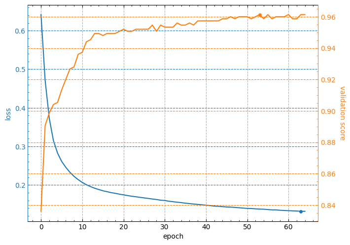
Note: the minimum value of loss curve and the maximum value of validation score curve are marked by points.
Customizing appearance of the output figure
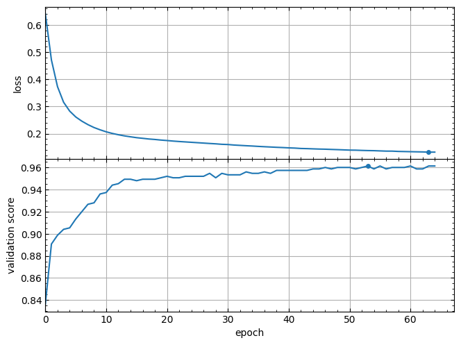
The lcurves_by_MLP_estimator function has optional parameters to customize the appearance of the output figure. For example,the lcurves_by_MLP_estimator function with on_separate_subplots=True shows the learning curves of loss and validation score on two separated subplots:
lcurves_by_MLP_estimator(clf, on_separate_subplots=True);
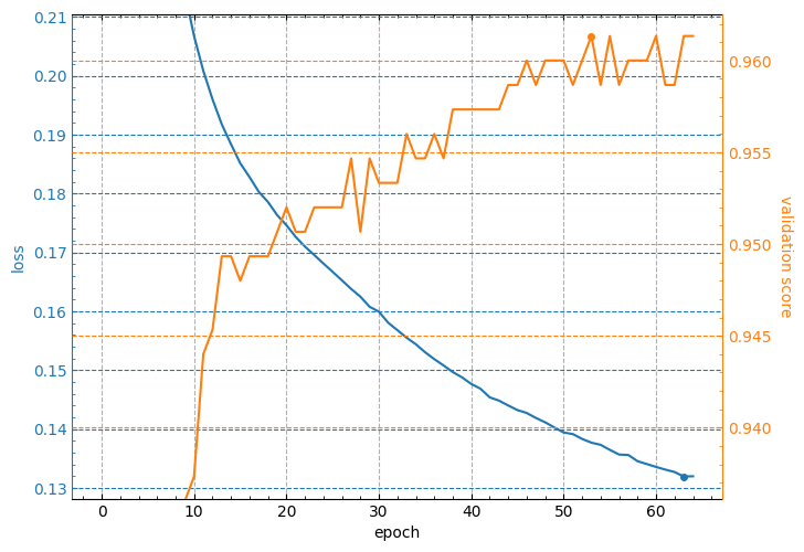
And the epoch_range_to_scale option allows to specify the epoch index range within which the subplots of the losses and metrics are scaled (see details about this option in the docstring of the lcurves_by_MLP_estimator function).
lcurves_by_MLP_estimator(clf, epoch_range_to_scale=10);
For a description of other optional parameters of the lcurves_by_MLP_estimator function to customize the appearance of the output figure, see its docstring.
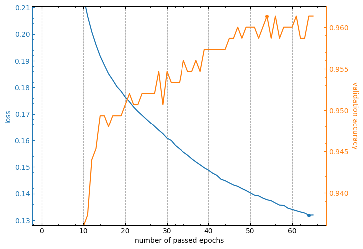
The lcurves_by_MLP_estimator function returns a numpy array or a list of the matplotlib.axes.Axes objects of an output figure (see additional details in the Returns section of the lcurves_by_MLP_estimator function docstring). So, you can use the methods of these objects to customize the appearance of the output figure.
axs = lcurves_by_MLP_estimator(clf, epoch_range_to_scale=11)
axs[0].grid(axis='y', visible=False)
axs[1].grid(axis='y', visible=False)
axs[0].set_xlabel('number of passed epochs')
axs[1].set_ylabel('validation accuracy');
CHANGELOG
All notable changes to this project will be documented in this file.
The format is based on Keep a Changelog, and this project adheres to Semantic Versioning.
[1.2.0] - 2026-05-05
Added
- A new boolean parameter
optimum_values_in_legendhas been added to thelcurves()function. The parameter specifies whether to display the optimum values of epochs and metrics in the legends of the the losses and metrics subplots.
[1.1.1] - 2026-02-26
Changed
- Improved x-axis tick placement logic in
lcurves()function for better readability of epoch numbers on the plot.
Fixed
- Small bug fixes.
[1.1.0] - 2026-01-24
Changed
- The
lcurves_by_history()function has been renamed tolcurves()to make the code easier to write and understand, butlcurves_by_history()remains as an alias for backward compatibility. - The
historyparameter of thelcurves()function has been renamed tohistories. It can now accept a list of dictionaries with several fitting histories of keras models.
Added
- Support for correct recognition of key names in learning history of model training with the Ultralytics YOLO library.
- Support for plotting multiple histories on a single figure using
lcurves()function. - The default value of the
initial_epochparameter of thelcurvesfunction has been changed from 0 to 1. - New parameters in
lcurves():color_grouping_by: Controls curve color grouping in subplots.model_names: Customizes legend labels for each history.optimization_modes: Sets metric optimization direction ("min"/"max")
- New
utilsmodule with utility functions:get_mode_by_metric_name(): Determines metric optimization mode.get_best_epoch_value(): Finds optimal epoch value.history_concatenate(): Concatenates two histories into one. The function was moved from thelcurvetoolsmodule to theutilsmodule, but it remained available for import from the mainlcurvetoolspackage module.
[1.0.1] - 2025-01-23
Changed
The default value for the figsize parameter of the lcurves_by_history() and lcurves_by_MLP_estimator() functions has been changed to None.
[1.0.0] - 2024-01-22
Initial release.


Download files
Download the file for your platform. If you're not sure which to choose, learn more about installing packages.
Source Distribution
Built Distribution
Filter files by name, interpreter, ABI, and platform.
If you're not sure about the file name format, learn more about wheel file names.
Copy a direct link to the current filters
File details
Details for the file lcurvetools-1.2.0.tar.gz.
File metadata
- Download URL: lcurvetools-1.2.0.tar.gz
- Upload date:
- Size: 24.8 kB
- Tags: Source
- Uploaded using Trusted Publishing? No
- Uploaded via: twine/4.0.2 CPython/3.11.9
File hashes
| Algorithm | Hash digest | |
|---|---|---|
| SHA256 |
d52b1022b01ff05b0f9814a147d51ea9b23c70e967ab4134e0f804e0b850afe7
|
|
| MD5 |
acf8f30eb1bb3dc96e108c0c30b5a761
|
|
| BLAKE2b-256 |
f5844f7144057e873a169ff56cc136c2f1ec394c7dbdb388985977c866f77cae
|
File details
Details for the file lcurvetools-1.2.0-py3-none-any.whl.
File metadata
- Download URL: lcurvetools-1.2.0-py3-none-any.whl
- Upload date:
- Size: 19.5 kB
- Tags: Python 3
- Uploaded using Trusted Publishing? No
- Uploaded via: twine/4.0.2 CPython/3.11.9
File hashes
| Algorithm | Hash digest | |
|---|---|---|
| SHA256 |
fcc9ca54f78070658d9fc5d0cc565af77a41ec9a048a68524be026deea902e54
|
|
| MD5 |
aa6693ec6350c19928c03f9124bac446
|
|
| BLAKE2b-256 |
6419c46b86a4c26bfcd0c84a5511d1fa3a73bddcb7d731e3ca2efb6807783e94
|


