
learned
Machine Learning library for Python
Introduction
Package containing deep learning model, classic machine learning models, various preprocessing functions and result metrics
Table of Contents
-
.neural_network
-
Sequential Class
-
DNNModel Class
-
Layer Class
-
.models
-
KNN class
-
LinReg class
-
LogReg class
-
GradientDescent class
-
.preprocessing
-
OneHotEncoder class
-
normalizer() function
-
get_split_data() function
-
polynomial_features() function
-
.metrics
-
confusion_matrix() function
-
accuracy() function
.neural_network
Explanation: It contains the classes required for the deep neural network. These classes can be customized with various functions. The trained model can be saved as a folder, then call this folder and used to predict other entries
Sequential class
Explanation:
		This class is used to create a sequential deep learning structure.

Parameters:
		x:
			Input values, as type below
		For example, if you select images for input values and the input data contains 30 sample images in 28x28 size,
	the images should be flattened to (pixel x N_sample), converted to (784, 30) and then entered into the model.
		y:
			Data which size of (1 x N_samples) for regression or (class_number x N_samples) for classification
		Note that: It can be (1 x N_samples) for binary classification. (if output layer contains sigmoid function)

Hyperparameters:
		learning_rate:
			It can be changed in case of exploding or vanishing of gradients. (Default value is 0.01)
		iteration:
			Iteration number. (Default value is 1000)
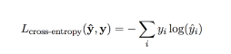
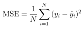
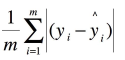
		loss:
			The loss function to be applied to the model is specified. (Default value is "binary_cross_entropy")
			Speciable loss functions:
				For classifications:
					"binary_cross_entropy" :

"cross_entropy" :
				For regressions:
					"mean_square_error" :
"mean_absolute_error" :
methods:
		Sequential.add(x):
			Adds a layer to the model structure.
			(x is a object which includes "Layer" class (very soon also "Convolution" class))

		Sequential.train():
			It starts the learning process and does not take parameters.

		Sequential.test(x, y):
			It gives the accuracy value for the test inputs and test outputs

		Sequential.predict(x):
			Returns the predicted value / category for x value

		Sequential.save_model("model_name"):
			Saves the trained model as a folder as specified in the parameter name. (To the same directory)

		Sequential.cost_list:
			It gives the costs for visualisation

		Sequential.accuracy_list:
			It gives the accuracies for visualisation
DNNModel class
Explanation:
		This class loads saved models

Parameters:
		model_folder: it takes saved model's folder name

Methods:
		DNNModel.predict(x):
			Returns the predicted value / category for x value
Layer class
Explanation:
		ANN model's hidden layers are defined by this layer

Hyperparameters:
		neurons:
			Indicates how many neurons the layer has

		weights_initializer:
			Determines how layer weights are started (default value is "uniform")
				"he_uniform":
						suitable_size_uniform_values * sqrt(6 / prev_layers_output_size)

				"he_normal":
						suitable_size_uniform_values * sqrt(2 / prev_layers_output_size)

				"xavier_uniform":
						suitable_size_uniform_values * sqrt(6 / (prev_layers_output_size + layer_neurons_size))

				"xavier_normal":
						suitable_size_uniform_values * sqrt(2 / (prev_layers_output_size + layer_neurons_size))

				"uniform":
						suitable_size_uniform_values * 0.1

				Note that: "he" initializers better for relu / leaky_relu activation functions

		activation:
			Determines with which function the layer will be activated. (default values is "tanh")
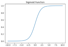
				"sigmoid": 0 - 1
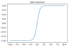
"tanh": -1 - 1
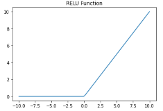
"relu": it makes all negative values to zero
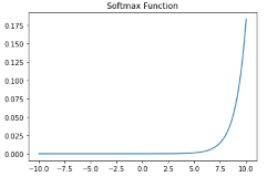
"softmax": it is a probability function, it return values which sums of values equal 1
"leaky_relu": it don't makes all negative values to zero but makes too close to zero
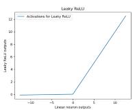
	Example for neural network structure:
				from learned.neural_network.models import Sequential, DNNModel
				from learned.neural_network.layers import Layer
				from learned.preprocessing import get_split_data, normalizer, OneHotEncoder

				mnist = pd.read_csv("train.csv")
				mnist.head()
				train, test = get_split_data(mnist, test_percentage=0.33)
				print(train.shape)
				>>> (28140, 785)
				y_labels_tr = train[:, :1]
				y_labels_te = test[:, :1]
				pixels_tr = train[:, 1:]
				pixels_te = test[:, 1:]
				pixels_tr = normalizer(pixels_tr)
				pixels_te = normalizer(pixels_te)
				pixels_tr = pixels_tr.T
				pixels_te = pixels_te.T
				print(pixels_tr.shape)
				>>> (784, 28140)
				ohe_tr = OneHotEncoder(y_labels_tr).transform()
				ohe_te = OneHotEncoder(y_labels_te).transform()

				Model = Sequential(pixels_tr, ohe_tr, learning_rate=0.01, loss="cross_entropy", iteration=600)

				Model.add(Layer(neurons=150, activation="relu", weights_initializer="he_normal"))
				Model.add(Layer(neurons=150, activation="relu", weights_initializer="he_normal"))
				Model.add(Layer(neurons=150, activation="relu", weights_initializer="he_normal"))
				Model.add(Layer(neurons=10, activation="softmax", weights_initializer="xavier_normal"))

				Model.train()

>>> pred2 == pred
.models
KNN class
Explanation:
	Includes the k-Nearest Neighbors algorithm.
Parameters:
	x:
		Train input values
	y:
		Train output values
Hyperparameters:
	k_neighbors:
		It determines how many neighbors will be evaluated.

	metric:
		"euclidean"
		It determines which distance finding function will be used.(Default value is "euclidean")
		(other distance functions coming soon)

	model:
		"classification" for categorical prediction
		"regression" for numerical prediction
Methods:
	KNN.predict(x):
		Returns prediction from K nearest neighbors. Returns the most frequently value for "classification" or
		returns average value for "regression"

Usage:
'''
	from learned.models import KNN
	knn = KNN(x, y, k_neighbors=3, metric="euclidean", model="classification")
	knn.predict(test_x)
'''
LinReg class
	Explanation:
        	LinReg is a class that allows simple or multiple linear regressions and returns trained parameters.

	Parameters:
        	data_x:
		Input values
    	data_y:
		True output values
	Usage:
	'''
	from learned.models import LinReg
	lin_reg = LinReg(data_x, data_y)
	'''
	Methods:

    	LinReg.train():
		It applies the training process for the dataset entered while creating the class.
		Output:
		(An example simple linear regression output)
		    '''
		    Completed in 0.0 seconds.
		    Training R2-Score: % 97.0552464372771
		    Intercept: 10349.456288746507, Coefficients: [[812.87723722]]
		    '''

	LinReg.test(test_x, test_y)
        		Applies the created model to a different input and gives the r2 score result.
	Output:
		(An example simple linear regression output)
		    '''
		    Testing R2-Score: % 91.953582170654
		    '''
		Note:
			Returns an error message if applied for a model that has not been previously trained.
			'''
			  Exception: Model not trained!
			'''

	LinReg.predict(x):
		Applies the created model to the input data, which it takes as a parameter, and returns the estimated results.

			Note:
		    Returns an error message if applied for a model that has not been previously trained.
		    '''
		    Exception: Model not trained!
		    '''
	LinReg.r2_score(y_true, y_predict)
        		It takes actual results and predicted results for the same inputs as parameters and returns the value of r2 score.

	LinReg.intercept
        		Returns the trained intercept value

	LinReg.coefficients
		Returns the trained coefficients
LogReg class
Explanation:
        	LogReg is a class that allows simple logistic regressions and returns trained parameters.
	Works as a neural network one layer which includes single perceptron

	Parameters:
        	x:
		Input values
    	y:
		True output values

Hyperparameters:
	learning_rate:
		It can be changed in case of exploding or vanishing of gradients. (Default value is 0.01)
	iteration:
		Iteration number. (Default value is 1000)
	Usage:
	'''
	from learned.models import LogReg
	log_reg = LogReg(x, y, learning_rate=0.001, iteration=1000)
	'''
	Methods:

    	LogReg.train():
		It applies the training process for the dataset entered while creating the class.

	LogReg.predict(x):
		Applies the created model to the input data, which it takes as a parameter, and returns the estimated results.

	LogReg.accuracy(y_true, y_pred):
		Gives the model accuracy value
GradientDescent class
	Explanation:
        	GradientDescent is a class that allows simple or multiple linear regressions and returns trained parameters.
	Works as a neural network one layer which includes single perceptron

	Parameters:
        	data_x:
		Input values
    	data_y:
		True output values
Hyperparameters:
	learning_rate:
		It can be changed in case of exploding or vanishing of gradients. (Default value is 0.00001)
	Usage:
	'''
	from learned.models import GradientDescent
	gd = GradientDescent(data_x, data_y, learning_rate=0.001)
	'''
	Methods:

    	GradientDescent.optimizer(number_of_steps=False):
		It applies the training process for the dataset entered while creating the class.

	Parameters:
		number_of_steps:
			Iteration number. Default value is "False".
			If no value is entered, continues until the step size is less than 0.0001.
		Output:
		(An example multiple linear regression output)
		    '''
		    Completed in 109.72 seconds
		    R-Squared:%63.32075249528732
		    Test Score: %41.059223927525004
		    (-17003.943940164645, array([[3349.00019104],
		    [1658.35639114],[  12.87388237]]))
		    '''

	GradientDescent.test(data_x, data_y):
        		Applies the created model to a different input and gives the r2 score result.

	GradientDescent.predict(x):
		Applies the created model to the input data, which it takes as a parameter, and returns the estimated results.

	GradientDescent.r2_score(y_true, y_pred)
        		It takes actual results and predicted results for the same inputs as parameters and returns the value of r2 score.

	GradientDescent.get_parameters():
		Returns the trained weights
.preprocessing
OneHotEncoder class
Explanation:
	One hot encoding is a process by which categorical variables are converted
into a form that could be provided to ML algorithms to do a better job in prediction.

Methods:
	OneHotEncoder(x).transform():
		Note: x must be a numpy object.
		Returns the transformed values.(Values are in ascending order / alphabetical order.)

	OneHotEncoder(x).values:
		Returns the dict which includes values and tranformed values
Usage:
'''
	from learned.preprocessing import OneHotEncoder
	ohe = OneHotEncoder(x)
'''
	For example,
		from learned.preprocessing import OneHotEncoder
		vals = ["cat", "dog", "bird", "lion"]
		ohe = OneHotEncoder(vals)
		transformed_vals = ohe.transform()
		transformed_vals => [[0, 1, 0, 0],
				     [0, 0, 1, 0],
				     [1, 0, 0, 0],
				     [0, 0, 0, 1]]
		the_dict = ohe.values
		the_dict => {"bird": [1, 0, 0, 0],
			     "cat":  [0, 1, 0, 0],
			     "dog":  [0, 0, 1, 0],
			     "lion": [0, 0, 0, 1]}
normalizer() function
Explanation:
	Converts the entered data to the 0-1 range.

Parameters:
	data:
		Entered data must be numpy object
Usage:
'''
	from learned.preprocessing import normalizer

	data = [1, 2, 3, 4, 5, 6, 7, 8, 9, 10]
	normalize = normalizer(data)
	normalize => [0.1, 0.2, 0.3, 0.4, 0.5, 0.6, 0.7, 0.8, 0.9, 1]
'''
get_split_data() function
Explanation:
	Divides and shuffles the given data.

Parameters:
	data:
		Full data (inputs and outputs (not split))
Hyperparameters:
	test_percentage:
		Determines what percentage of data is allocated as test data.(Default value is 0.33)
	random_state:
		Determines the random distribution constant.(Default value is 0)

Usage:
'''
	from learned.preprocessing import get_split_data

	train_data, test_data = get_split_data(full_data, test_percentage=0.2, random_state=42)
'''
polynomial_features() function
Explanation:
	Adds polynomial features, layers to the entered data.

Parameters:
	data:
		Input data
Hyperparameters:
	degree:
		It determines the degree of polynomial distribution to be made.(Default value is "2")
Usages:
'''
	from learned.preprocessing import polynomial_features

	a = np.array([[1, 2], [3, 4], [6, 2], [2, 7]])
	features = polynomial_features(a, degree=3)
	features => [[  1.   2.   1.   2.   4.   1.   2.   4.   8.]
		     [  3.   4.   9.  12.  16.  27.  36.  48.  64.]
		     [  6.   2.  36.  12.   4. 216.  72.  24.   8.]
	 	     [  2.   7.   4.  14.  49.   8.  28.  98. 343.]]
'''
.metrics
confusion_matrix() function
Explanation:
	Returns the confusion matrix of the entered data. Operates on both categorical and regression values.
	Entries must be of (class_numbers x N_samples) size for categorical data, and (1 x N_samples) for regression data.

Parameters:
	y_true:
		Real output
	y_pred:
		Predicted output
Usage:
'''
	from learned.metrics import confusion_matrix
	y_true = np.array([[0, 1, 1, 2, 0, 2, 1, 3]])
	y_pred = np.array([[0, 0.8, 0, 1.2, 1, 2, 1, 2.6]])
	print(confusion_matrix(y_true, y_pred))
	=> [[1, 1, 0, 0],
	    [1, 2, 1, 0],
	    [0, 0, 1, 0],
	    [0, 0, 0, 1]]
'''
accuracy() function
Explanation:
	Returns the accuracy value for the given values.

Parameters:
	y_true:
		Real output
	y_pred:
		Predicted output
Usage:
'''
	from learned.metrics import accuracy
	y_true = np.array([[0, 1, 1, 2, 0, 2, 1, 3]])
	y_pred = np.array([[0, 0.8, 0, 1.2, 1, 2, 1, 2.6]])
	print(accuracy(y_true, y_pred))
	=> 0.625 (% 62.5)
'''
TODO
- cross validation
- p-value
- Other algorithms
- Examples
1 maintainer

Metadata
1 maintainer
Release files for learned 0.5.4.5
For a detailed explanation of source distributions (sdists) and built distributions (wheels), please see the package formats documentation.
Source distribution (sdist)
| File | Size | Uploaded | |
|---|---|---|---|
| learned-0.5.4.5.tar.gz | 19.6 kB | Details |
Built distribution (wheel)
| File | Interpreter | ABI | Platform | Reset |
|---|---|---|---|---|
| learned-0.5.4.5-py3-none-any.whl | Python 3 | none | any | Details |
Total release size: 35.1 kB
Release files / learned-0.5.4.5.tar.gz
| Download URL | learned-0.5.4.5.tar.gz |
|---|---|
| Size | 19.6 kB |
| Tags | Source |
|
SHA-256 checksum How to use checksums |
b5efb9a6b3ec1850335e62816d4abce12a33e83f8e000fc7d0cebb850678b472
|
|
BLAKE2b-256 checksum How to use checksums |
a617570ae0bb0e6034b5c729ba9d8bc9fd0519d00cbfedc6ed5f0b54639ba56a
|
| Upload date | |
|
Uploaded using Trusted Publishing? What is trusted publishing? |
No |
| Uploaded via |
twine/3.4.1 importlib_metadata/3.10.0 pkginfo/1.6.1 requests/2.24.0 requests-toolbelt/0.9.1 tqdm/4.50.2 CPython/3.8.5
|
Release files / learned-0.5.4.5-py3-none-any.whl
| Download URL | learned-0.5.4.5-py3-none-any.whl |
|---|---|
| Size | 15.5 kB |
| Tags | Python 3 |
|
SHA-256 checksum How to use checksums |
09b92ac25e96a63db027fb37a095f26e7b09638034f1e222dd72ed9942608486
|
|
BLAKE2b-256 checksum How to use checksums |
bc3c07ba3b4f244c5c133cfd57a7eaf8e9e415d961af4f30c257e2381972297c
|
| Upload date | |
|
Uploaded using Trusted Publishing? What is trusted publishing? |
No |
| Uploaded via |
twine/3.4.1 importlib_metadata/3.10.0 pkginfo/1.6.1 requests/2.24.0 requests-toolbelt/0.9.1 tqdm/4.50.2 CPython/3.8.5
|














