Monocular 3D pose Estimation on Laboratory Animals

Project description
LiftPose3D
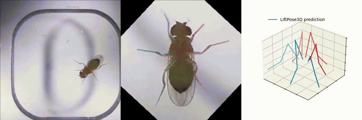
LiftPose3D is a tool for transforming a 2D poses to 3D coordinates on labaratory animals. Classical approaches based on triangulation require synchronised acquisition from multiple cameras and elaborate calibration protocols. By contrast, LiftPose3D can reconstruct 3D poses from 2D poses from a single camera, in some instances without having to know the camera position or the type of lens used. For the theoretical background and details, have a look at our paper.
To train LiftPose3D, ideally you would need (A) a 3D pose library, (B) corresponding 2D poses from the camera that you will use for lifting and (C) camera matrices (extrinsic and intrinsic).
If you do not have access to
- (A) then use one of the provided datasets,
- (B) then obtain 2D images via projection using your camera matrices (you will need to calibrate to obtain these)
- (C) then place your camera further away to assume weak perspective.
Starting-Up
Data format
During training, LiftPose3D accepts two numpy arrays in shape of [N J 2] and [N J 3] serving as input and output. Here, N is the number of poses and J is the number of joints. If you have multiple experiments, you can provide your data as dictionaries where the keys are strings and values are numpy arrays. You will also need the set at least one root joint and a set of target sets for each root joint. The network will predict the joints in the target sets relative to the root joints.
For each example, we provide a unique load.py file to transform data into the required [N J 3] LifPose3D format.
Training
You can train a network with the following generic syntax using experiment 1 for training and experiment 2 for testing.
from liftpose.main import train as lp3d_train
import numpy.random.rand

n_points, n_joints = 100, 5
train_2d, test_2d = rand((n_points, n_joints, 2)), rand((n_points, n_joints, 2))
train_3d, test_3d = rand((n_points, n_joints, 3)), rand((n_points, n_joints, 3))

train_2d = {"experiment_1": train_2d}
train_3d = {"experiment_1": train_3d}
test_2d = {"experiment_2": test_2d}
test_3d = {"experiment_2": test_3d}

roots = [0]
target_sets = [1,2,3,4]

lp3d_train(train_2d, test_2d, train_3d, test_3d, roots, target_sets)
By default, the outputs will be saved in a folder out relative to the path where LiftPose3D is called. You can change this behavior using the ouput_folder parameter of the train function. You can take a look at the train function for other default values and much longer documentation here.
For example, you can further configure training by passing an extra argument training_kwargs in train function.
from liftpose.main import train as lp3d_train
training_kwargs={ "epochs": 15,                   # train for 15 epochs
                  "resume": True,                 # resume training where it was stopped
                  "load"  : 'ckpt_last.pth.tar'}, # use last training checkpoint to resume

lp3d_train(train_2d, test_2d, train_3d, test_3d, roots, target_sets, training_kwargs=training_kwargs)
You can overwrite all the parameter inside liftpose.lifter.opt using training_kwargs.
Training augmentation
Augmenting training data is a great way to account for variability in the dataset, especially when training data is scarce.
Currently, available options in liftpose.lifter.augmentation are:
add_noise: adding Gaussian noise on 2D training pose to account for uncertainty in test timerandom_project: random projections of 3D pose in case camera orientation is unknown during test time (the training will ignore the inputtrain_2d)perturb_pose: pose augmentation by changing segment lengths when there are large animal-to-animal variationproject_to_cam: deterministic projections of 3D pose in case camera matrix is different and known in test time
Training augmentation options can be specified in the argument augmentation and can be combined.
from liftpose.main import train as lp3d_train
from liftpose.lifter.augmentation import random_project

angle_aug = {'eangles' : {0: [[-10,10], [-10, 10], [-10,10]]}, #range of Euler angles (dictionary indexed by an integer which specifies the camera identify)
             'axsorder': 'zyx', # order of rotations for euler angles
             'vis'     : None,  # used in case not all joints are visible from a given camera
             'tvec'    : None,  # camera translation vector
             'intr'    : None}  # camera intrinsic matrix

aug = [random_project(**angle_aug)]
lp3d_train(train_2d, test_2d, train_3d, test_3d, roots, target_sets, aug=aug)
See the case of angle invariant Drosophila lifting for an example implementation of augmentation.
Inspecting the training
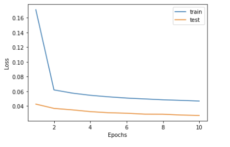
The training information is saved under the train_log.txt, which can be visualized as follows.
from liftpose.plot import read_log_train, plot_log_train
epoch, lr, loss_train, loss_test, err_test = read_log_train(par['out_dir'])
plot_log_train(plt.gca(), loss_train, loss_test, epoch)
This will plot the training and test losses during the training.
Testing the network
To test the network on the data provided during the lp3d_train call, run
from liftpose.main import test as lp3d_test
lp3d_test(par['out_dir'])
Results will be saved inside the test_results.pth.tar file.
To test the network in new data, run
liftpose3d_test(par['out_dir'], test_2d, test_3d)
where you provide the test_2d and test_3d in the format described above. This will overwrite the previous test_results.pkl file, if there is any.
We also provide a simple interface for loading the test results from the test_results.pkl file.
from liftpose.postprocess import load_test_results
test_3d_gt, test_3d_pred, _ = load_test_results(par['out_dir'])
This will return two numpy arrays: test_3d_gt, which is the same as test_3d, and test_3d_pred, which has the predictions from the LiftPose3D.
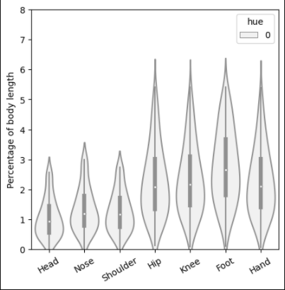
To generate the error distribution run
 from liftpose.plot import violin_plot

 names = ['Head', 'Nose', 'Shoulder',  'Hip',  'Knee', 'Foot', 'Hand']
 violin_plot(plt.gca(), test_3d_gt=test_3d_gt, test_3d_pred=test_3d_pred, test_keypoints=np.ones_like(test_3d_gt),
             joints_name=names, units='m', body_length=2.21)
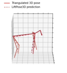
Visualizing the 3D pose
To visualize the output 3D pose, first specify an animal skeleton in the file params.yaml. Note that bone information or the connected joints, are only used for visualization and not during training. You can have a closer look at plot_pose_3d function to see how the bone and color parameters are used during plotting.
data:
    roots       : [0]
    target_sets : [[1, 2, 3, 4]]

vis:
    colors      : [[186, 30, 49]]
    bones       : [[0, 1], [1, 2], [2, 3], [3, 4]]
    limb_id     : [0, 0, 0, 0, 0]
We provide the following function to visualize the 3D data
from liftpose.plot import plot_pose_3d
fig = plt.figure(figsize=plt.figaspect(1), dpi=100)
ax = fig.add_subplot(111, projection='3d')
ax.view_init(elev=-75, azim=-90)

t = 0
plot_pose_3d(ax=ax, tar=test_3d_gt[t],
           pred=test_3d_pred[t],
           bones=par_data["vis"]["bones"],
           limb_id=par_data["vis"]["limb_id"],
           colors=par_data["vis"]["colors"],
           legend=True)
This should output something similar to:
You can also easily create movies
from liftpose.plot import plot_video_3d

fig = plt.figure(figsize=plt.figaspect(1), dpi=100)
ax = fig.add_subplot(111, projection='3d')

ax.set_xlim([-4,2])
ax.set_ylim([-3,2])
ax.set_zlim([0,2])

plot_video_3d(fig, ax, n=gt.shape[0], par=par_data, tar=gt, pred=pred, trailing=10, trailing_keypts=[4,9,14,19,24,29], fps=20)
Use trailing to plot points trailing_keypts with a trailing effect with a desired length.
Training with subset of points
In case you want to prevent some 2D/3D points from used in the training, you can pass train_keypts argument into the train function, which has the same shape as train_3d but has boolean datatype. Alternatively, in case you have missing keypoints, you can convert them to np.NaN. In both cases, the loss from these points is not going to be used during backpropagation.
Release history Release notifications | RSS feed


Download files
Download the file for your platform. If you're not sure which to choose, learn more about installing packages.
Source Distribution
Built Distribution
Filter files by name, interpreter, ABI, and platform.
If you're not sure about the file name format, learn more about wheel file names.
Copy a direct link to the current filters
File details
Details for the file liftpose-0.22.tar.gz.
File metadata
- Download URL: liftpose-0.22.tar.gz
- Upload date:
- Size: 34.6 kB
- Tags: Source
- Uploaded using Trusted Publishing? No
- Uploaded via: twine/3.4.1 importlib_metadata/3.10.0 pkginfo/1.7.0 requests/2.24.0 requests-toolbelt/0.9.1 tqdm/4.50.2 CPython/3.6.12
File hashes
| Algorithm | Hash digest | |
|---|---|---|
| SHA256 |
9994756752d983386850fb99dab000ddf4c3bbbed1806288cd6c83495f02ef55
|
|
| MD5 |
392235721bf90bdbd09fe9493853deab
|
|
| BLAKE2b-256 |
ed56d8538dd68175fa58d413e1ebe6c69af9982ba12027d436aee2f4d98e202a
|
File details
Details for the file liftpose-0.22-py3-none-any.whl.
File metadata
- Download URL: liftpose-0.22-py3-none-any.whl
- Upload date:
- Size: 48.4 kB
- Tags: Python 3
- Uploaded using Trusted Publishing? No
- Uploaded via: twine/3.4.1 importlib_metadata/3.10.0 pkginfo/1.7.0 requests/2.24.0 requests-toolbelt/0.9.1 tqdm/4.50.2 CPython/3.6.12
File hashes
| Algorithm | Hash digest | |
|---|---|---|
| SHA256 |
4b78cdae95b7d1f6c1b3682dafcd979319ebb411a3f2dae89faf878610e6b4ba
|
|
| MD5 |
2b46fbd13d209a1766c4e58aff7e763f
|
|
| BLAKE2b-256 |
a6b9491b5c593b5ddcf42d1be17add7156824c45dfc0d428876ec5ba9a6219f5
|


