Package for Media-Mix-Modelling

Project description

Lightweight (Bayesian) Marketing Mix Modeling
LMMM is a python library that helps organisations understand and optimise marketing spend across media channels.
This is not an official Google product.


Docs • Introduction • Theory • Getting Started • References • Community Spotlight
Introduction
Marketing Mix Modeling (MMM) is used by advertisers to measure advertising effectiveness and inform budget allocation decisions across media channels. Measurement based on aggregated data allows comparison across online and offline channels in addition to being unaffected by recent ecosystem changes (some related to privacy) which may affect attribution modelling. MMM allows you to:
- Estimate the optimal budget allocation across media channels.
- Understand how media channels perform with a change in spend.
- Investigate effects on your target KPI (such as sales) by media channel.
Taking a Bayesian approach to MMM allows an advertiser to integrate prior information into modelling, allowing you to:
- Utilise information from industry experience or previous media mix models using Bayesian priors.
- Report on both parameter and model uncertainty and propagate it to your budget optimisation.
- Construct hierarchical models, with generally tighter credible intervals, using breakout dimensions such as geography.
The LightweightMMM package (built using Numpyro and JAX) helps advertisers easily build Bayesian MMM models by providing the functionality to appropriately scale data, evaluate models, optimise budget allocations and plot common graphs used in the field.
Theory
Simplified Model Overview
An MMM quantifies the relationship between media channel activity and sales, while controlling for other factors. A simplified model overview is shown below and the full model is set out in the model documentation. An MMM is typically run using weekly level observations (e.g. the KPI could be sales per week), however, it can also be run at the daily level.
$$kpi = \alpha + trend + seasonality + media\ channels + other\ factors$$
Where kpi is typically the volume or value of sales per time period, $\alpha$ is the model intercept, $trend$ is a flexible non-linear function that captures trends in the data, $seasonality$ is a sinusoidal function with configurable parameters that flexibly captures seasonal trends, $media\ channels$ is a matrix of different media channel activity (typically impressions or costs per time period) which receives transformations depending on the model used (see Media Saturation and Lagging section) and $other\ factors$ is a matrix of other factors that could influence sales.
Standard and Hierarchical models
The LightweightMMM can either be run using data aggregated at the national level (standard approach) or using data aggregated at a geo level (sub-national hierarchical approach).
-
National level (standard approach). This approach is appropriate if the data available is only aggregated at the national level (e.g. The KPI could be national sales per time period). This is the most common format used in MMMs.
-
Geo level (sub-national hierarchical approach). This approach is appropriate if the data can be aggregated at a sub-national level (e.g. the KPI could be sales per time period for each state within a country). This approach can yield more accurate results compared to the standard approach because it uses more data points to fit the model. We recommend using a sub-national level model for larger countries such as the US if possible.
Media Saturation and Lagging
It is likely that the effect of a media channel on sales could have a lagged effect which tapers off slowly over time. Our powerful Bayesian MMM model architecture is designed to capture this effect and offers three different approaches. We recommend users compare all three approaches and use the approach that works the best. The approach that works the best will typically be the one which has the best out-of-sample fit (which is one of the generated outputs). The functional forms of these three approaches are briefly described below and are fully expressed in our model documentation.
- Adstock: Applies an infinite lag that decreases its weight as time passes.
- Hill-Adstock: Applies a sigmoid like function for diminishing returns to the output of the adstock function.
- Carryover: Applies a causal convolution giving more weight to the near values than distant ones.
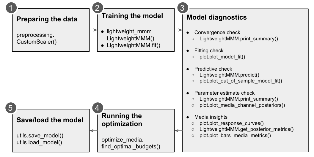
Flow chart
Getting started
Installation
The recommended way of installing lightweight_mmm is through PyPi:
pip install --upgrade pip
pip install lightweight_mmm
If you want to use the most recent and slightly less stable version you can install it from github:
pip install --upgrade git+https://github.com/google/lightweight_mmm.git
If you are using Google Colab, make sure you restart the runtime after installing.
Preparing the data
Here we use simulated data but it is assumed you have your data cleaned at this point. The necessary data will be:
- Media data: Containing the metric per channel and time span (eg. impressions per time period). Media values must not contain negative values.
- Extra features: Any other features that one might want to add to the analysis. These features need to be known ahead of time for optimization or you would need another model to estimate them.
- Target: Target KPI for the model to predict. For example, revenue amount, number of app installs. This will also be the metric optimized during the optimization phase.
- Costs: The total cost per media unit per channel.
# Let's assume we have the following datasets with the following shapes (we use
the `simulate_dummy_data` function in utils for this example):
media_data, extra_features, target, costs = utils.simulate_dummy_data(
    data_size=160,
    n_media_channels=3,
    n_extra_features=2,
    geos=5) # Or geos=1 for national model
Scaling is a bit of an art, Bayesian techniques work well if the input data is small scale. We should not center variables at 0. Sales and media should have a lower bound of 0.
ycan be scaled asy / jnp.mean(y).mediacan be scaled asX_m / jnp.mean(X_m, axis=0), which means the new column mean will be 1.
We provide a CustomScaler which can apply multiplications and division scaling
in case the wider used scalers don't fit your use case. Scale your data
accordingly before fitting the model.
Below is an example of usage of this CustomScaler:
# Simple split of the data based on time.
split_point = data_size - data_size // 10
media_data_train = media_data[:split_point, :]
target_train = target[:split_point]
extra_features_train = extra_features[:split_point, :]
extra_features_test = extra_features[split_point:, :]

# Scale data
media_scaler = preprocessing.CustomScaler(divide_operation=jnp.mean)
extra_features_scaler = preprocessing.CustomScaler(divide_operation=jnp.mean)
target_scaler = preprocessing.CustomScaler(
    divide_operation=jnp.mean)
# scale cost up by N since fit() will divide it by number of time periods
cost_scaler = preprocessing.CustomScaler(divide_operation=jnp.mean)

media_data_train = media_scaler.fit_transform(media_data_train)
extra_features_train = extra_features_scaler.fit_transform(
    extra_features_train)
target_train = target_scaler.fit_transform(target_train)
costs = cost_scaler.fit_transform(unscaled_costs)
In case you have a variable that has a lot of 0s you can also scale by the mean
of non zero values. For instance you can use a lambda function to do this:
lambda x: jnp.mean(x[x > 0]). The same applies for cost scaling.
Training the model
The model requires the media data, the extra features, the costs of each media unit per channel and the target. You can also pass how many samples you would like to use as well as the number of chains.
For running multiple chains in parallel the user would need to set
numpyro.set_host_device_count to either the number of chains or the number of
CPUs available.
See an example below:
# Fit model.
mmm = lightweight_mmm.LightweightMMM()
mmm.fit(media=media_data,
        extra_features=extra_features,
        media_prior=costs,
        target=target,
        number_warmup=1000,
        number_samples=1000,
        number_chains=2)
If you want to change any prior in the model (besides the media prior which you
are already specifying always), you can do so with custom_priors:
# See detailed explanation on custom priors in our documentation.
custom_priors = {"intercept": numpyro.distributions.Uniform(1, 5)}

# Fit model.
mmm = lightweight_mmm.LightweightMMM()
mmm.fit(media=media_data,
        extra_features=extra_features,
        media_prior=costs,
        target=target,
        number_warmup=1000,
        number_samples=1000,
        number_chains=2,
        custom_priors=custom_priors)
Please refer to our documentation on custom_priors for more details.
You can switch between daily and weekly data by enabling
weekday_seasonality=True and seasonality_frequency=365 or
weekday_seasonality=False and seasonality_frequency=52 (default). In case
of daily data we have two types of seasonality: discrete weekday and smooth
annual.
Model diagnostics
Convergence Check
Users can check convergence metrics of the parameters as follows:
mmm.print_summary()
The rule of thumb is that r_hat values for all parameters are less than 1.1.
Fitting check
Users can check fitting between true KPI and predicted KPI by:
plot.plot_model_fit(media_mix_model=mmm, target_scaler=target_scaler)
If target_scaler used for preprocessing.CustomScaler() is given, the target
would be unscaled. Bayesian R-squared and MAPE are shown in the chart.
Predictive check
Users can get the prediction for the test data by:
prediction = mmm.predict(
    media=media_data_test,
    extra_features=extra_data_test,
    target_scaler=target_scaler
)
Returned prediction are distributions; if point estimates are desired, users
can calculate those based on the given distribution. For example, if data_size
of the test data is 20, number_samples is 1000 and number_of_chains is 2,
mmm.predict returns 2000 sets of predictions with 20 data points. Users can
compare the distributions with the true value of the test data and calculate
the metrics such as mean and median.
Parameter estimation check
Users can get detail of the parameter estimation by:
mmm.print_summary()
The above returns the mean, standard deviation, median and the credible interval for each parameter. The distribution charts are provided by:
plot.plot_media_channel_posteriors(media_mix_model=mmm, channel_names=media_names)
channel_names specifies media names in each chart.
Media insights
Response curves are provided as follows:
plot.plot_response_curves(media_mix_model=mmm, media_scaler=media_scaler, target_scaler=target_scaler)
If media_scaler and target_scaler used for preprocessing.CustomScaler() are given, both the media and target values would be unscaled.
To extract the media effectiveness and ROI estimation, users can do the following:
media_effect_hat, roi_hat = mmm.get_posterior_metrics()
media_effect_hat is the media effectiveness estimation and roi_hat is the ROI estimation. Then users can visualize the distribution of the estimation as follows:
plot.plot_bars_media_metrics(metric=media_effect_hat, channel_names=media_names)
plot.plot_bars_media_metrics(metric=roi_hat, channel_names=media_names)
Running the optimization
For optimization we will maximize the sales changing the media inputs such that the summed cost of the media is constant. We can also allow reasonable bounds on each media input (eg +- x%). We only optimise across channels and not over time. For running the optimization one needs the following main parameters:
n_time_periods: The number of time periods you want to simulate (eg. Optimize for the next 10 weeks if you trained a model on weekly data).- The model that was trained.
- The
budgetyou want to allocate for the nextn_time_periods. - The extra features used for training for the following
n_time_periods. - Price per media unit per channel.
media_gaprefers to the media data gap between the end of training data and the start of the out of sample media given. Eg. if 100 weeks of data were used for training and prediction starts 2 months after training data finished we need to provide the 8 weeks missing between the training data and the prediction data so data transformations (adstock, carryover, ...) can take place correctly.
See below and example of optimization:
# Run media optimization.
budget = 40 # your budget here
prices = np.array([0.1, 0.11, 0.12])
extra_features_test = extra_features_scaler.transform(extra_features_test)
solution = optimize_media.find_optimal_budgets(
    n_time_periods=extra_features_test.shape[0],
    media_mix_model=mmm,
    budget=budget,
    extra_features=extra_features_test,
    prices=prices)
Save and load the model
Users can save and load the model as follows:
utils.save_model(mmm, file_path='file_path')
Users can specify file_path to save the model.
To load a saved MMM model:
utils.load_model(file_path: 'file_path')
Citing LightweightMMM
To cite this repository:
@software{lightweight_mmmgithub,
  author = {Pablo Duque and Dirk Nachbar and Yuka Abe and Christiane Ahlheim and Mike Anderson and Yan Sun and Omri Goldstein and Tim Eck},
  title = {LightweightMMM: Lightweight (Bayesian) Marketing Mix Modeling},
  url = {https://github.com/google/lightweight_mmm},
  version = {0.1.6},
  year = {2022},
}
References
Support
As LMMM is not an official Google product, the LMMM team can only offer limited support.
For questions about methodology, please refer to the References section or to the FAQ page.
For issues installing or using LMMM, feel free to post them in the Discussions or Issues tabs of the Github repository. The LMMM team responds to these questions in our free time, so we unfortunately cannot guarantee a timely response. We also encourage the community to share tips and advice with each other here!
For feature requests, please post them to the Discussions tab of the Github repository. We have an internal roadmap for LMMM development but do pay attention to feature requests and appreciate them!
For bug reports, please post them to the Issues tab of the Github repository. If/when we are able to address them, we will let you know in the comments to your issue.
Pull requests are appreciated but are very difficult for us to merge since the code in this repository is linked to Google internal systems and has to pass internal review. If you submit a pull request and we have resources to help merge it, we will reach out to you about this!
Community Spotlight
-
How To Create A Marketing Mix Model With LightweightMMM by Mario Filho.
-
How Google LightweightMMM Works and A walkthrough of Google’s LightweightMMM by Mike Taylor.
Release history Release notifications | RSS feed


Download files
Download the file for your platform. If you're not sure which to choose, learn more about installing packages.
Source Distribution
Built Distribution
Filter files by name, interpreter, ABI, and platform.
If you're not sure about the file name format, learn more about wheel file names.
Copy a direct link to the current filters
File details
Details for the file lightweight_mmm-0.1.9.tar.gz.
File metadata
- Download URL: lightweight_mmm-0.1.9.tar.gz
- Upload date:
- Size: 86.1 kB
- Tags: Source
- Uploaded using Trusted Publishing? No
- Uploaded via: twine/4.0.2 CPython/3.11.3
File hashes
| Algorithm | Hash digest | |
|---|---|---|
| SHA256 |
3f6562476f08dc30e10bdee569784782edaf79724ee34b64a525ce55e2fbf01c
|
|
| MD5 |
1707def11bb15e4e9867089510fb7fd7
|
|
| BLAKE2b-256 |
a4f8e62ca95469c338a8715b9bcde7b92af2f687e47900bf9f4a571a577a8a7a
|
File details
Details for the file lightweight_mmm-0.1.9-py3-none-any.whl.
File metadata
- Download URL: lightweight_mmm-0.1.9-py3-none-any.whl
- Upload date:
- Size: 105.2 kB
- Tags: Python 3
- Uploaded using Trusted Publishing? No
- Uploaded via: twine/4.0.2 CPython/3.11.3
File hashes
| Algorithm | Hash digest | |
|---|---|---|
| SHA256 |
cbf1dba6774710d54137334c76fa94b6a654b12476a79e30d904a97fe00a9899
|
|
| MD5 |
d667ef920163b11fdde71aee6341e36e
|
|
| BLAKE2b-256 |
e94f4de01b34a2b22303a0b694f98457632ea689767b5e79d0657898de8c2b37
|


