Toolbox for Eccentric BBH Populations and LISA Waveforms

Project description
leap: LISA Eccentricity Astrophysics Package
Xuan et al. (2026)
📖 Overview
LEAP (distributed on PyPI as lisa-leap) is a Python toolkit for generating eccentric compact binary populations and computing their gravitational wave signals in the LISA band. It supports population synthesis, waveform computation, and signal analysis, including:
📂 BBH Population Catalogs
Note: Each module provides methods such as sample merger eccentricities and generate population snapshots. The snapshot functions return a list of
CompactBinaryobjects.
-
🌌 Galactic Nuclei (GN): SMBH-perturbed mergers (steady-state & starburst)
- Based on: Hoang et al. (2018, ApJ 856, 140); Xuan et al. (2024a, ApJ 965, 148); Stephan et al. (2019, ApJ 878, 58)
-
✨ Globular Clusters (GC): Dynamically formed BBHs, including in-cluster and ejected mergers
- Based on: Kremer et al. (2020, ApJS 247, 48); Zevin et al. (2020, ApJ 903, 67); Xuan et al. (2025b, ApJL 985, L42)
-
🌠 Galactic Field: Fly-by–induced mergers in Milky Way–like and elliptical galaxies
- Based on: Michaely & Perets (2019, ApJL 887, L36); Raveh et al. (2022, MNRAS 514, 4246); Michaely & Naoz (2022, ApJ 936, 184); Xuan et al. (2024a, ApJ 965, 148)
🛠 Waveform & Signal Analysis
Note: Perform calculations via high-level
CompactBinaryobjects, OR input parameters directly into the Functional API:
- Generate PN-based, time-domain waveforms for eccentric binaries (via Class Method or Functional API). [Phys. Rev. D 82, 024033]
- Evolve orbital parameters throughout the inspiral stage (via Class Method or Functional API). [Peters 1964, Phys. Rev. 136, B1224]
- Compute the LISA detector response (Michelson signal) for a given GW waveform (via Functional API). [Phys. Rev. D 67, 022001]
- Evaluate characteristic strain ($h_c$) and stochastic backgrounds (via Class Method or Functional API). [Phys. Rev. D 110, 023020]
- Calculate signal-to-noise ratio (SNR) and noise-weighted inner products (via Class Method or Functional API).
💾 Installation
To install the latest version using pip, simply run the following in your terminal (Command Prompt / PowerShell on Windows, Terminal on macOS / Linux):
pip install lisa-leap
Then in Python:
import leap
Note for Mac/Linux: If pip is not found or defaults to Python 2, try pip3 instead:
pip3 install lisa-leap
Or, you can install the latest development version via GitHub. Please choose the method that matches your environment:
Method 1: Jupyter Notebook / Google Colab
If you are working in a notebook (Jupyter, Colab, Kaggle), run the following command in a code cell.
!pip install https://github.com/zeyuanxuan/lisa-leap/archive/refs/heads/main.zip
Method 2: Terminal / Command Line
If you are using a standard terminal, run the command without the !
pip install https://github.com/zeyuanxuan/lisa-leap/archive/refs/heads/main.zip
Note for Mac/Linux: If pip is not found or defaults to Python 2, try pip3 instead:
pip3 install https://github.com/zeyuanxuan/lisa-leap/archive/refs/heads/main.zip
Method 3: University Clusters / HPC
If you are running jobs on a cluster using existing Python modules (like module load python/3.9.6), load the same module before installing.
Step 1 — load the Python module you intend to use in your job script:
# Example: if your submission script uses python/3.9.6, load it now:
module load python/3.9.6
Step 2 — install the package with --user. This installs the package into your local directory specific to that Python version (e.g., ~/.local/lib/python3.9/site-packages).
python3 -m pip install --user https://github.com/zeyuanxuan/lisa-leap/archive/refs/heads/main.zip
Step 3 — import leap in your code and run your job:
# In your job script (.sh/.pbs):
module load python/3.9.6
python your_script.py
Updating to the Latest Version (from GitHub)
If you have previously installed lisa-leap from GitHub and want to pull the latest updates from the main branch, add the --upgrade, --no-cache-dir, and --force-reinstall flags to force a clean reinstallation:
pip install --upgrade --no-cache-dir --force-reinstall "https://github.com/zeyuanxuan/lisa-leap/archive/refs/heads/main.zip"
⚡ Quickstart
Once lisa-leap is installed, you can walk through the most common workflow below: build a Milky Way catalog, pick one binary from it, and then run the full signal-analysis pipeline (waveform → spectrum → characteristic strain → SNR) on that single source.
import leap
# -----------------------------------------------------------------
# 1. Generate a Milky Way eccentric-GW source catalog (Running this step may take some time)
# -----------------------------------------------------------------
mw_catalog = leap.getMWcatalog(plot=True, tobs_yr=10.0)
print(f"Catalog size: {len(mw_catalog)} systems")
# Each entry is [label, m1 (msun), m2 (msun), a (au), e, Dl (kpc), snr, metadata_dict].
# Pick the highest-SNR source for a detailed look:
best = max(mw_catalog, key=lambda row: row[6])
label, m1, m2, a, e, Dl, snr, meta = best
print(f"Brightest source: {label} | M={m1:.1f}+{m2:.1f} Msun, "
f"a={a:.3e} AU, e={e:.4f}, SNR={snr:.2f} for 10yr observation")
# -----------------------------------------------------------------
# 2. Wrap it as a CompactBinary object for analysis
# -----------------------------------------------------------------
binary = leap.CompactBinary(
m1=m1, m2=m2, a=a, e=e, Dl=Dl,
label=label
)
# -----------------------------------------------------------------
# 3. Time-domain waveform (h_+, h_x)
# -----------------------------------------------------------------
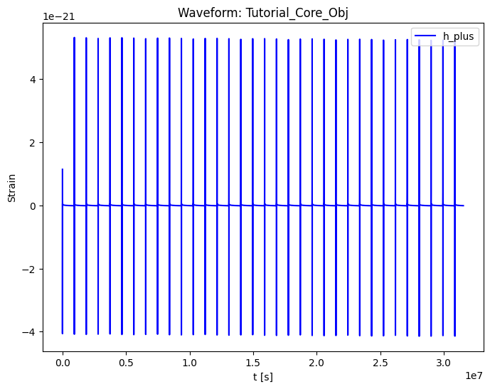
t_vec, h_plus, h_cross = binary.compute_waveform(
tobs_yr=0.5, points_per_peak=50, plot=True
)
# -----------------------------------------------------------------
# 4. Numerical spectrum (hc_num via FFT of the waveform above)
# -----------------------------------------------------------------
f_axis, hc_num = binary.get_spectrum(
tobs_yr=0.5, polarization='hplus', plot=True
)
# -----------------------------------------------------------------
# 5. Characteristic strain (analytic, non-evolving limit)
# -----------------------------------------------------------------
freq, hc_env, hc_insp, hc_nonevolve, snr_contrib = \
binary.compute_characteristic_strain(tobs_yr=4.0, plot=True)
# -----------------------------------------------------------------
# 6. Sky-averaged SNR (full harmonic integration)
# -----------------------------------------------------------------
snr_val = binary.compute_snr_analytical(tobs_yr=4.0)
print(f"4-year sky-averaged SNR = {snr_val:.2f}")
For deeper control (custom populations, LISA response, noise curve swaps, numerical inner product, etc.), see the corresponding sections in §3–§5 below.
🚀 If you simply want to get a catalog...
📥 Pre-generated catalog available: If you don't want to run the generator yourself, a pre-computed catalog of 10 Milky Way realizations is shipped with the repository and can be downloaded directly here:
MW_BBH_catalog_10realizations.csv. You can also download it from theGithub webpage. Each row follows the same schema as thegetMWcatalog()return value (see below), so you can load it withpandasornumpyand plug the rows intoCompactBinary.from_list(row, schema='snapshot_std')for downstream analysis.
Or, you can use the all-in-one getMWcatalog() function.
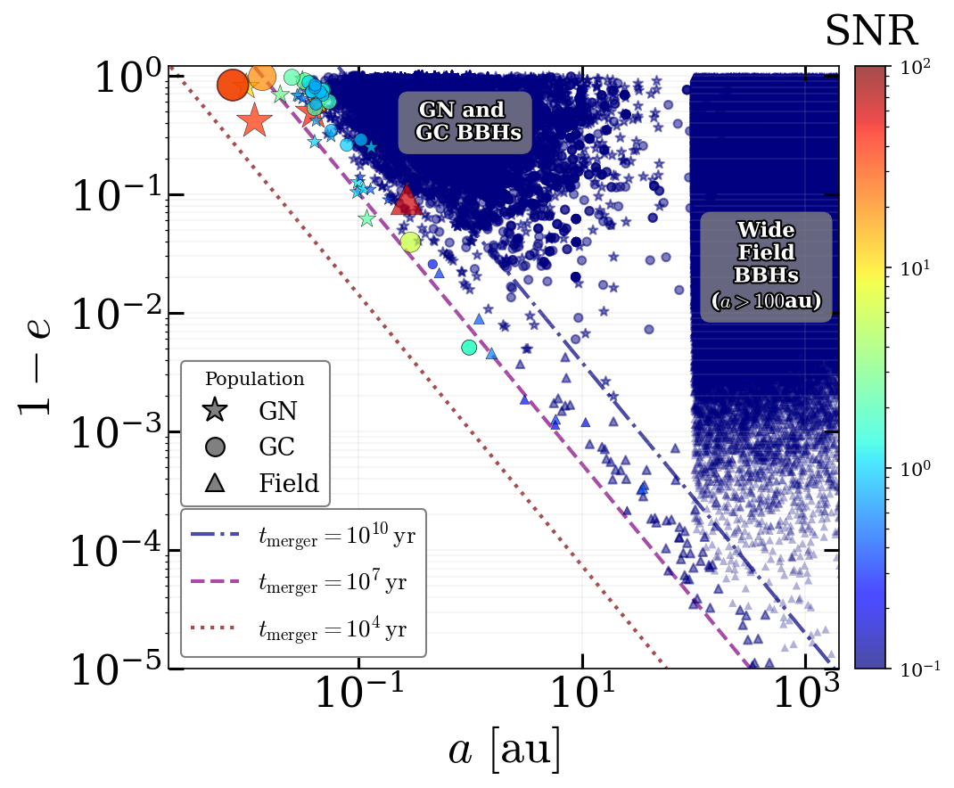
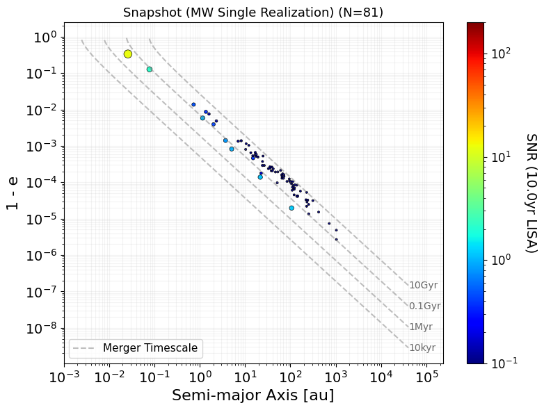
This feature randomly generates snapshot populations from all three formation environments in the Milky Way (Galactic Nuclei, Globular Clusters, and the Galactic Field), estimates their analytical SNRs, and visualizes the entire population in a single scatter plot.
leap.getMWcatalog()
- Input:
plot(bool, optional): IfTrue, generates a $1-e$ vs. $a$ scatter plot of the entire Milky Way catalog. Default isTrue.include_field_bkg(bool, optional): IfTrue, incorporates the background wide-field binaries into the catalog (which are largely irrelevant to the mHz GW source catalog but useful as a visual reference). Default isFalse.bkg_pct(float, optional): Fraction of the background wide-field-binaries population to simulate (e.g.,0.01for 1%). Default is0.01.tobs_yr(float, optional): Observation time in years used for SNR calculation. Default is10.0.
- Output:
- A list of generated binary systems. Each element is formatted as:
[label, m1, m2, a, e, Dl, snr, metadata_dict]. Themetadata_dictpreserves the detailed physical origin (e.g., specific globular cluster names, orGN_YNC/GN_steadystate) under the'source_label'key.
- A list of generated binary systems. Each element is formatted as:
Example:
import leap

# Generate the full Milky Way catalog and plot it
mw_catalog = leap.getMWcatalog(
    plot=True,
    include_field_bkg=True,
    bkg_pct=0.01,
    tobs_yr=10.0
)

# Inspect the first system in the catalog
first_system = mw_catalog[0]
label, m1, m2, a, e, Dl, snr, metadata = first_system

print(f"\nPopulation size: {len(mw_catalog)} systems")
print(f"Sample System [{label}]: m1={m1} M_sun, m2={m2} M_sun, a={a:.4e} AU, e={e:.4f}")
print(f"Original Source: {metadata.get('source_label', 'Unknown')}")
- Output (approximate — exact counts depend on stochastic realization and the shipped Field aggregate file):
 Population size: 735084 systems
 Sample System [GN]: m1=10.82333 M_sun, m2=8.562529 M_sun, a=1.2974e-01 AU, e=0.2276
 Original Source: GN_Steadystate
🎯 Features & Usage Examples
1️⃣ Global Configuration
leap.set_output_control
Sets the global verbosity and warning suppression levels.
- Input:
verbose(bool): IfFalse, disables internal library printing.show_warnings(bool): IfFalse, suppresses warnings (e.g.,RuntimeWarning).
- Output:
None.
Example:
# Silence both stdout prints and warnings from internal routines
leap.set_output_control(verbose=False, show_warnings=False)
2️⃣ CompactBinary Class
The core class of the package. Each object represents a single binary system, managing its physical properties, orbital evolution, waveform generation, and data storage.
leap.CompactBinary()
To create a binary system object:
- Input:
m1,m2(float): Masses [$M_\odot$].a(float): Semi-major axis [au].e(float): Eccentricity (0 <= e < 1).Dl(float): Luminosity distance [kpc].label(str): Identifier string (free-form).extra(dict, optional): Dictionary for storing extended parameters (e.g., SNR, inclination [rad], spin, lifetime). Analysis methods that derive quantities (e.g.compute_fpeak,compute_merger_time,compute_snr_analytical) will also write their results here.
- Output:
CompactBinaryobject.
Example:
my_binary = leap.CompactBinary(
    m1=10.0, m2=10.0, a=0.26, e=0.985, Dl=8.0,
    label="Tutorial_Core_Obj",
    extra={
        'inclination': 0.7854,  # [rad] (~45 degrees)
    }
)
print(f"   Output Object: {my_binary}")
print(f"   Type Inspection: {type(my_binary)}")
# You can also access extra data directly
print(f"   Inclination: {my_binary.extra['inclination']:.4f} rad")
- Output:
 Output Object: <CompactBinary [Tutorial_Core_Obj]: M=10.0+10.0 m_sun, a=2.600e-01AU, e=0.9850, Dl=8.0kpc | inclination=0.785>
 Type Inspection: <class 'leap.core.CompactBinary'>
 Inclination: 0.7854 rad
.to_list() .from_list()
Methods to convert CompactBinary objects to and from list formats, facilitating data storage (e.g., to CSV/NumPy files) and retrieval.
- .to_list():
- Input:
schema(str) — formatting standard (default:'snapshot_std', i.e.,[label, Dl, a, e, m1, m2, snr]). Thesnrvalue is read fromself.extra['snr'](defaults to0.0if absent). - Output: A list representing the system's data.
- Input:
- .from_list() (classmethod):
- Input:
data_list(list) — raw values;schema(str) — one of'snapshot_std','gn_prog','field_prog'. For'field_prog', masses must be supplied viaaux_params={'m1': ..., 'm2': ...}since the row itself does not carry them. - Output: A new
CompactBinaryobject instantiated from the list.
- Input:
Example:
# Export
print("   A. to_list(schema='snapshot_std')")
data_row = my_binary.to_list(schema='snapshot_std')
print(f"      Output: {data_row} (Type: List)")

# Import
print("   B. from_list(data_list=..., schema='snapshot_std')")
raw_in = ["Imp_Sys", 16.8, 0.5, 0.9, 50.0, 50.0, 0.0]
new_obj = leap.CompactBinary.from_list(data_list=raw_in, schema='snapshot_std')
print(f"      Output: {new_obj}")
- Output:
A. to_list(schema='snapshot_std')
  Output: ['Tutorial_Core_Obj', 8.0, 0.26, 0.985, 10.0, 10.0, 0.0] (Type: List)
B. from_list(data_list=..., schema='snapshot_std')
  Output: <CompactBinary [Imp_Sys]: M=50.0+50.0 m_sun, a=0.50AU, e=0.9000, Dl=16.8kpc, snr=0.000>
.compute_merger_time()
Calculates the remaining time until the merger due to gravitational wave emission (Peters 1964 formula).
- Input:
verbose(bool, optional): Controls standard output printing. Default isTrue.
- Output:
t_merge_yr(float): Time to merger in years.- Note: The result is also stored in
self.extra['merger_time_yr'].
Example:
t_merge_yr = my_binary.compute_merger_time(verbose=False)
print(f"      Return Value: {t_merge_yr:.4e} [years] (Type: float)")
- Output:
Return Value: 4.8407e+06 [years] (Type: float)
.compute_snr_analytical()
Computes the sky-averaged Signal-to-Noise Ratio (SNR) for the LISA detector. This method supports the full integration of harmonics (default) and a fast geometric approximation. It also incorporates the time-evolving integration for systems that chirp significantly during the observation.
- Input:
tobs_yr(float): Observation duration in years.quick_analytical(bool, optional):- If
False(default): Uses full integration (summing over harmonics viaPN_waveform.SNR). - If
True: Uses a fast geometric approximation based on peak frequency and amplitude, suitable for high-$e$ systems with slow evolution.
- If
force_evolve(bool, optional): Force the use of the time-evolving SNR integration regardless of the merger timescale. Only effective whenquick_analytical=False. DefaultFalse.evolve_threshold(float, optional): Threshold ratio that triggers the time-evolving integration automatically. Whent_merger < evolve_threshold * tobs, the system is considered to be evolving significantly during the observation and the evolving integral is used instead of the static-source one. Only effective whenquick_analytical=False. Default10.0.n_segments(int, optional): Number of log-spaced time segments used by the evolving SNR integral. Segments are denser near merger where orbital evolution is fastest. Default100.f_orb_max_Hz(float, optional): Orbital-frequency upper cutoff [Hz]. The evolving integration stops once $f_{\rm orb}$ exceeds this value, since by then the source has left the LISA band and further SNR contributions are negligible. Default0.1.verbose(bool, optional): Controls standard output printing. Default isTrue.
- Output:
snr_val(float): The calculated SNR value.- Note: The result is also stored in
self.extra['snr_analytical'].
- Notes:
- Branch selection (when
quick_analytical=False):- If
force_evolve=True, ORt_merger < evolve_threshold * tobs, the method uses the time-evolving integral: the orbit is propagated via Peters (1964) equations along $N$ log-spaced segments from $t=0$ to $\min(t_{\rm obs}, t_{\rm merger})$, each segment contributes $d{\rm SNR}^2$ assuming the midpoint orbital parameters are static, and the total is $\sqrt{\sum d{\rm SNR}^2}$. - Otherwise (slow-evolution regime), the method falls back to the original static-source full-harmonic integration (
PN_waveform.SNR), which assumes the orbit is essentially frozen during $t_{\rm obs}$.
- If
- The evolving branch automatically truncates the integration once the orbital frequency exceeds
f_orb_max_Hz(default 0.1 Hz). This avoids numerical issues very close to merger and costs no SNR (the band is already gone). - If the system's merger time is shorter than
tobs_yr, the effective observation time is capped at $t_{\rm merger}$ in all branches.
- Branch selection (when
Example:
# Default: full integration, auto-switches to evolving if t_merger < 10 * tobs
snr_val = my_binary.compute_snr_analytical(tobs_yr=4.0, verbose=False)
print(f"      Return Value: {snr_val:.4f} (Type: float)")

# Force the time-evolving integral (useful for fast-chirping systems)
snr_val_evolve = my_binary.compute_snr_analytical(
    tobs_yr=4.0, force_evolve=True, n_segments=500, verbose=False
)

# Quick geometric approximation
snr_val_quick = my_binary.compute_snr_analytical(
    tobs_yr=4.0, quick_analytical=True, verbose=False
)
- Output:
Return Value: 10.9644 (Type: float)
.compute_fpeak()
Calculates the peak gravitational wave frequency ($f_{\rm peak}$) for the eccentric binary using the Wen (2003) approximation: $$f_{\rm peak} \approx f_{\rm orb} \cdot \frac{(1+e)^{1.1954}}{(1-e)^{1.5}} , .$$
Note: This follows the convention of Wen 2003 eq. 36 — it is the frequency of the peak-power harmonic expressed in terms of $f_{\rm orb}$, not the circular-orbit GW frequency $2f_{\rm orb}$.
- Input:
verbose(bool, optional): Controls standard output printing. Default isTrue.
- Output:
f_peak(float): Peak GW frequency [Hz].- Note: The result is also stored in
self.extra['f_peak_Hz'].
Example:
f_peak = my_binary.compute_fpeak(verbose=False)
print(f"      Return Value: {f_peak:.4e} [Hz] (Type: float)")
- Output:
Return Value: 1.3205e-03 [Hz] (Type: float)
.evolve_orbit()
Predicts the future state of the binary system by evolving its orbital parameters forward in time due to gravitational wave emission (Peters 1964 formula). Supports negative delta_t_yr for inverse evolution.
- Input:
delta_t_yr(float): Time duration to evolve the system, in years.update_self(bool, optional):- If
True: Updates theaandeattributes of theCompactBinaryobject itself. - If
False(default): Returns the new values without modifying the object.
- If
verbose(bool, optional): Controls standard output printing.
- Output:
(a_new, e_new)tuple:a_new(float): Evolved semi-major axis [au].e_new(float): Evolved eccentricity.
Example:
a_new, e_new = my_binary.evolve_orbit(delta_t_yr=1000.0, update_self=False, verbose=False)
print(f"      Return Tuple: a={a_new} au, e={e_new}")
- Output:
Return Tuple: a=0.25991616861323 au, e=0.9849951873952284
.compute_waveform()
A convenience method to compute the Gravitational Wave (GW) waveform specifically for the initialized binary system. It automatically uses the object's internal physical attributes ($m_1, m_2, a, e, D_L$) and supports adaptive time sampling.
- Input:
- Observation:
tobs_yr(float): Observation duration in years.initial_orbital_phase(float, optional): Initial mean anomaly $l_0$ [rad]. Default0.
- Source Geometry:
theta(float, optional): Line-of-sight polar angle in source frame [rad]. Default $\pi/4$.phi(float, optional): Line-of-sight azimuthal angle in source frame [rad]. Default $\pi/4$.
- Physics Model:
PN_orbit(int, optional): PN order for conservative orbital dynamics (0, 1, 2, 3). Default3.PN_reaction(int, optional): PN order for radiation reaction (0, 1, 2). Default2.
- Computational Control:
ts(float, optional): Fixed sampling time step [s]. IfNone(default), uses adaptive sampling.points_per_peak(int, optional): Resolution for adaptive sampling (points per periastron passage). Default50.max_memory_GB(float, optional): Safety limit for array size in GB. Default16.0.
- Output Control:
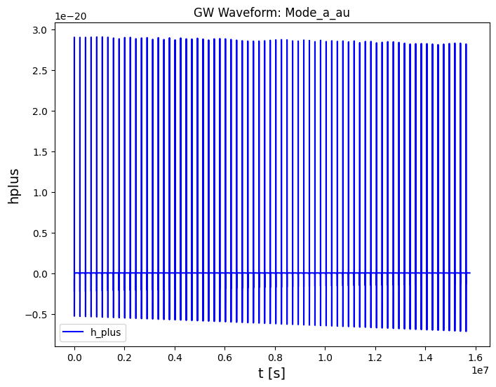
plot(bool, optional): IfTrue, plots $h_+$.verbose(bool, optional): Controls standard output printing.
- Observation:
- Output:
- A list of three NumPy arrays:
[time_vector, h_plus, h_cross]. ReturnsNoneif calculation fails.
- A list of three NumPy arrays:
- Notes:
- If the merger time is shorter than
tobs_yr, the waveform is truncated at ISCO. e = 0is not supported by the eccentric PN template (singularities in PN terms). It is automatically reset to1e-5with a printed warning.
- If the merger time is shorter than
Example:
wf_data_obj = my_binary.compute_waveform(
    tobs_yr=1.0, points_per_peak=50, verbose=False, plot=True
)
- Output:
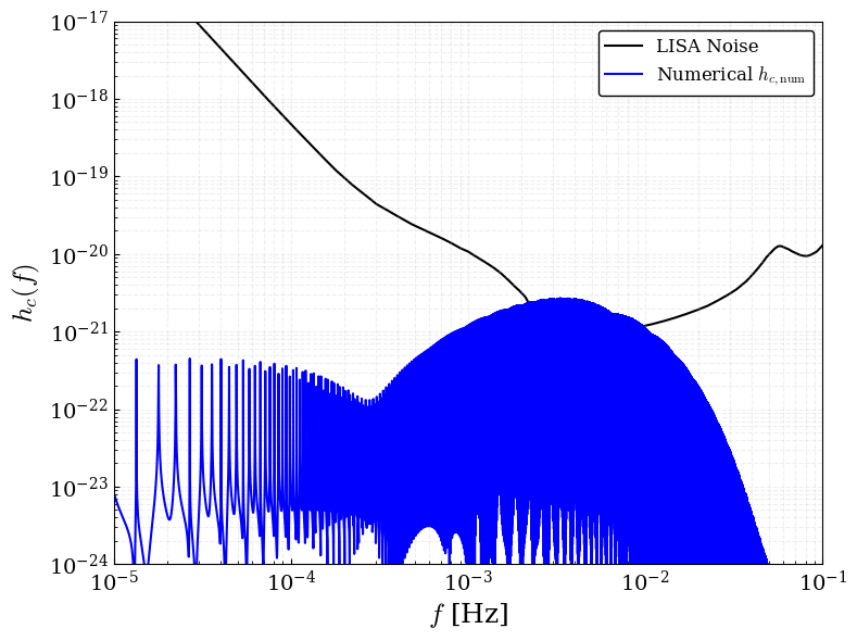
.get_spectrum()
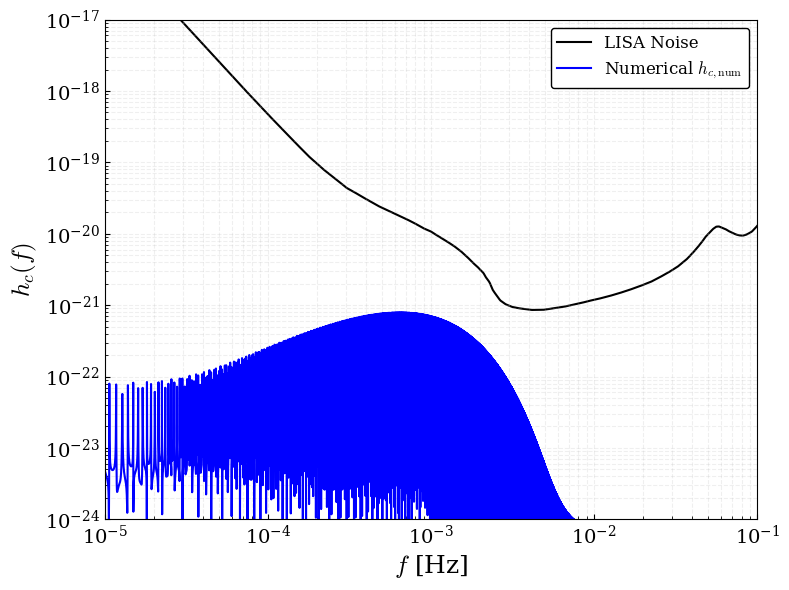
Automatically generates the time-domain waveform for the binary system and computes its numerical spectrum representation ($h_{c, \mathrm{num}}$) via Fast Fourier Transform (FFT).
-
Physics Note (Ref: Appendix A.3 of Xuan et al. 2026): In the non-evolving limit ($\dot{f} \to 0$), the comb-like peak heights of the numerical spectrum ($h_{c, \mathrm{num}}$) coincide with the discrete harmonic representation ($h_{c, \mathrm{non\text{-}evolve}}$). Because the smoothed spectrum ($h_{c, \mathrm{env}}$) redistributes energy to preserve the integrated SNR, these numerical peaks will appear lower than the smoothed envelope by a factor of $\sqrt{f_{\mathrm{orb}}/f}$.
-
Input:
- Observation & Signal:
tobs_yr(float): Observation duration in years.polarization(str, optional): Waveform polarization to analyze ('hplus'or'hcross'). Default'hplus'.theta,phi(float, optional): Sky position angles [rad]. Default $\pi/4$.initial_orbital_phase(float, optional): Initial mean anomaly [rad]. Default0.
- Sampling & Control:
ts(float, optional): Fixed sampling time step [s]. IfNone(default), adaptive sampling is used and the equivalent rate is recovered automatically for the FFT.points_per_peak(int, optional): Resolution for adaptive sampling. Default50.PN_orbit,PN_reaction(int, optional): PN orders. Default3,2.plot(bool, optional): IfTrue, plots the numerical characteristic strain against the LISA noise curve.verbose(bool, optional): Controls standard output printing.
- Observation & Signal:
-
Output:
- A
tupleof two NumPy arrays:(freq_axis, hc_num).[0] freq_axis: Frequency axis [Hz] (positive half-space).[1] hc_num: Numerical characteristic strain spectrum ($h_{c, \mathrm{num}}$).
- A
Example:
# Extract the spectrum directly from a CompactBinary object
f_axis, hc_num = my_binary.get_spectrum(
    tobs_yr=1.0,
    ts=5.0,                 # 5-second sampling interval
    polarization='hplus',   # analyze the plus polarization
    plot=True
)

print(f"   Output: Tuple of 2 Elements")
print(f"      [0] Frequency Axis     (shape: {f_axis.shape})")
print(f"      [1] Numerical Spectrum (shape: {hc_num.shape})")
- Output:
   Output: Tuple of 2 Elements
      [0] Frequency Axis     (shape: (315360,))
      [1] Numerical Spectrum (shape: (315360,))
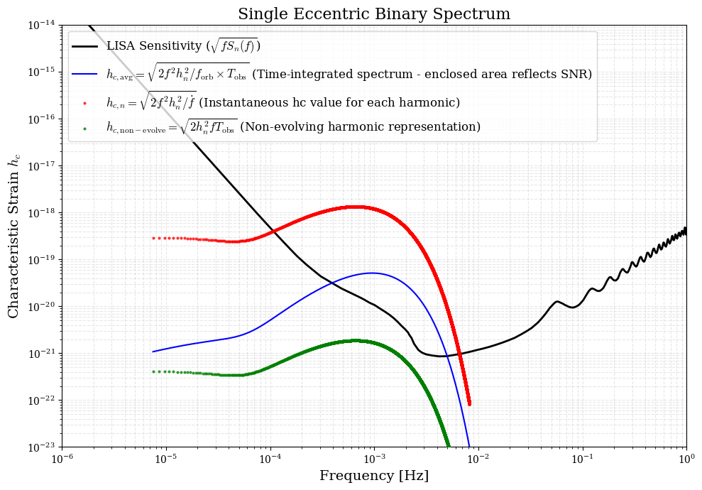
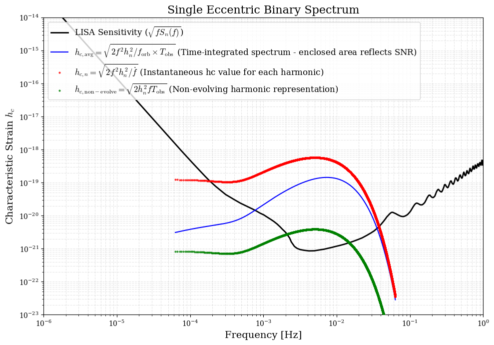
.compute_characteristic_strain()
Computes the characteristic strain spectrum ($h_c$) for the binary system. This method provides different physically equivalent representations of the characteristic strain; see Appendix A.2 and A.3 of Xuan et al. (2026) for details.
Note: This fast calculation method assumes the binary's evolution is negligible during the observation. For systems with significant chirp during
tobs_yr, use.compute_characteristic_strain_evolve()instead.
-
Input:
tobs_yr(float): Integration time in years.plot(bool, optional): IfTrue, generates a spectrum plot.
-
Output:
-
A list of 5 NumPy arrays:
[freq, hc_spectrum, hc_harmonics, hc_non_evolve, snr_contrib].-
[0] freq: Frequency list [Hz]. -
[1] hc_spectrum: Smoothed spectrum representation ($h_{c,\mathrm{env}}(f)$). Formula: $h_{c,\mathrm{env}} = \sqrt{2}, h_n \sqrt{f T_{\mathrm{obs}}} \sqrt{f / f_{\mathrm{orb}}}$. This continuous envelope redistributes the power of discrete harmonics over frequency space so that the area between it and the noise curve in a log–log plot directly reflects the integrated SNR. -
[2] hc_harmonics: Individual harmonic representation ($h_{c,\mathrm{insp}}$). Formula: $h_{c,\mathrm{insp}} = \sqrt{2}, h_n \sqrt{f^2 / \dot{f}}$. Pre-integration (evolving) characteristic strain amplitude of individual harmonics. -
[3] hc_non_evolve: Non-evolving / discrete harmonic representation ($h_{c,\mathrm{non\text{-}evolve}}$). Formula: $h_{c,\mathrm{non\text{-}evolve}} = \sqrt{2}, h_n \sqrt{f T_{\mathrm{obs}}}$. Post-integration peak height of each discrete harmonic assuming $\dot{f} \to 0$.In practice, they are combined as: $h_c = \sqrt{2}, h_n \sqrt{ \min( f^2 / \dot{f},; f T_{\mathrm{obs}} ) }$.
-
[4] snr_contrib: Contribution to the noise power spectral density $S_n(f)$ at harmonic frequencies.
-
-
Example:
strain_res_list = my_binary.compute_characteristic_strain(tobs_yr=4.0, plot=True)
- Output:
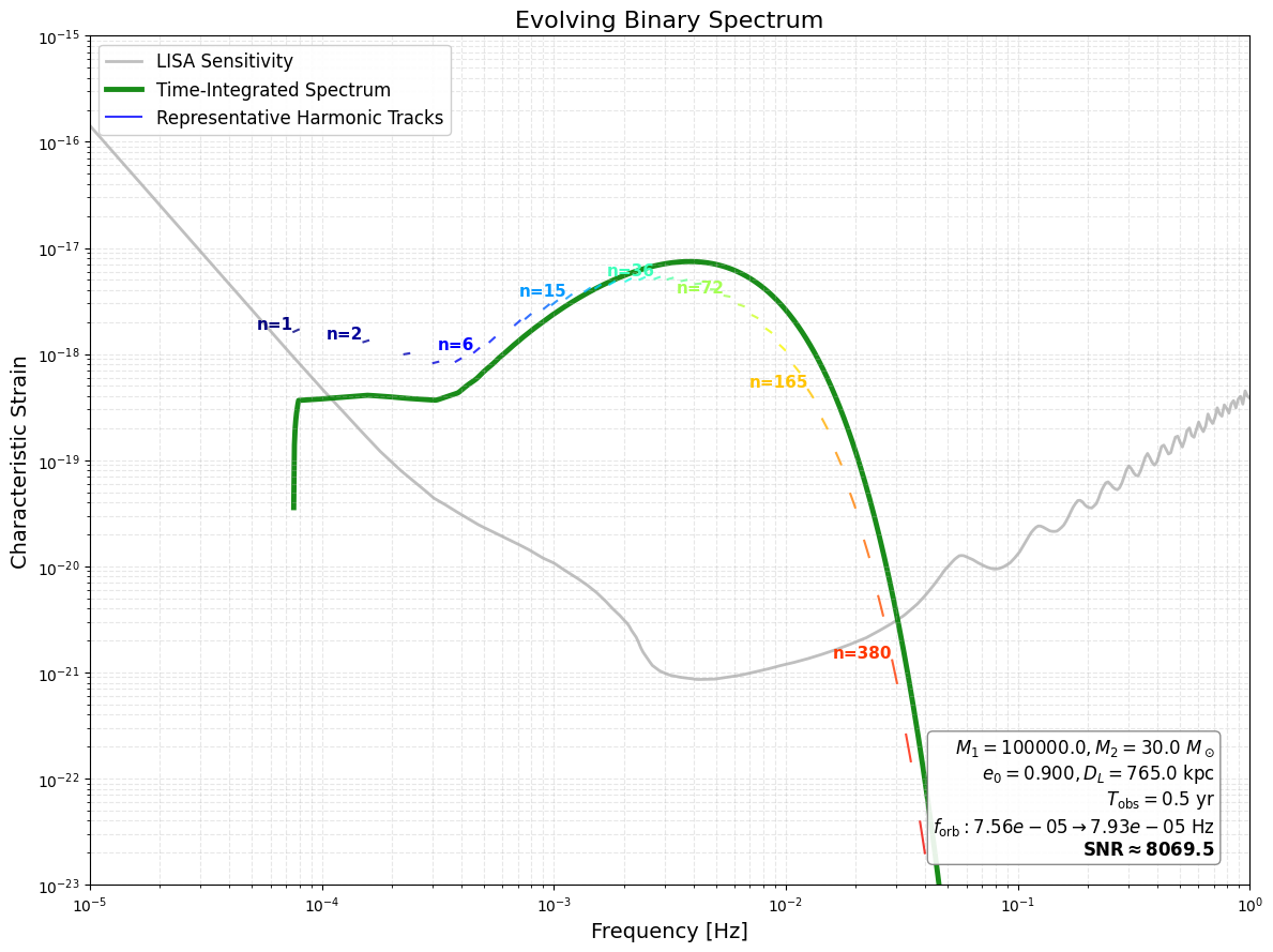
.compute_characteristic_strain_evolve()
Computes the time-evolving characteristic strain spectrum ($h_c$) by integrating the signal along the binary's evolutionary track (Peters 1964 equations). This method captures the "chirping" of harmonics across the frequency band.
Note: Unlike
.compute_characteristic_strain(), this handles significant orbital evolution (chirping) during the observation window.
-
Input:
tobs_yr(float): Integration time in years.target_n_points(int, optional): Number of harmonics to track for visualization. Default100. Ignored ifall_harmonics=True.all_harmonics(bool, optional):False(default): Uses optimized high-density sampling for spectrum integration and sparse sampling for plotting tracks. Fast and visually clear.True: Forces calculation of all integer harmonics within the band. Slower but rigorous.
plot(bool, optional): IfTrue, generates a plot showing both the instantaneous harmonic tracks and the total integrated spectrum.verbose(bool, optional): Controls standard output printing.
-
Output:
- A list of 4 elements:
[freq, hc_spectrum, snapshots, snr].[0] freq: Unified frequency axis [Hz] (log-spaced).[1] hc_spectrum: Total time-integrated characteristic strain ($h_{c,\rm avg}$) accumulated over $T_{\rm obs}$.[2] snapshots: A list of dictionaries, where each dictionary represents the system's state at a specific time step (containingt,f_orb,n,freq,hnc).[3] snr: The integrated SNR calculated from the spectrum.
- A list of 4 elements:
Example:
my_binary_evolve = leap.CompactBinary(
    m1=1e5, m2=30.0,
    a=0.26, e=0.9, Dl=765.0,
    label="Evolving_Source_Example"
)
evolve_res = my_binary_evolve.compute_characteristic_strain_evolve(
    tobs_yr=0.5,
    target_n_points=50,
    all_harmonics=False,
    plot=True,
    verbose=True
)
if evolve_res is not None:
    f_axis, hc_total, snapshots, snr = evolve_res
    print(f"\n   Output Inspection (List of 4 Elements):")
    print(f"      [0] Unified Frequency Axis (shape: {f_axis.shape})")
    print(f"          - Range: {f_axis[0]:.1e} Hz to {f_axis[-1]:.1e} Hz")
    print(f"      [1] Total Integrated Strain (h_c) (shape: {hc_total.shape})")
    print(f"          - Peak Amplitude: {np.max(hc_total):.4e}")
    print(f"      [2] Snapshots List (Length: {len(snapshots)})")
    print(f"          - Contains time-step details (t, f_orb, e, n, hnc...)")
    print(f"          - Example Keys: {list(snapshots[0].keys()) if len(snapshots)>0 else 'Empty'}")
    print(f"      [3] Integrated SNR (float)")
    print(f"          - Value: {snr:.4f}")
- Output:
 Output Inspection (List of 4 Elements):
    [0] Unified Frequency Axis (shape: (2000,))
        - Range: 1.0e-06 Hz to 1.0e+00 Hz
    [1] Total Integrated Strain (h_c) (shape: (2000,))
        - Peak Amplitude: 7.4468e-18
    [2] Snapshots List (Length: 100)
        - Contains time-step details (t, f_orb, e, n, hnc...)
        - Example Keys: ['t', 'f_orb', 'n', 'freq', 'hnc']
    [3] Integrated SNR (float)
        - Value: 8069.5495
3️⃣ Population analysis
3.1 Galactic Nuclei (GN)
This module models Binary Black Holes formed dynamically in Milky Way–like galactic nuclei (due to the perturbation of a central supermassive black hole). It is based on detailed three-body simulations.
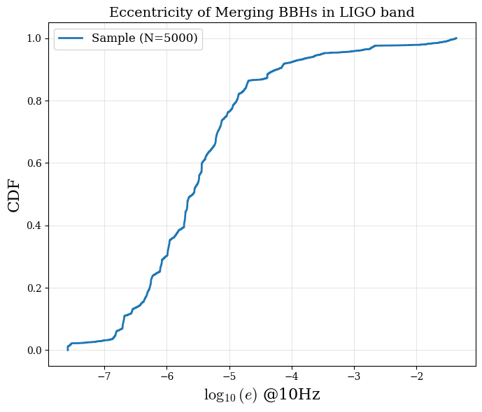
leap.GN.sample_eccentricities()
Randomly samples $N$ merger eccentricities for BBHs formed in Galactic Nuclei, defined at the LIGO frequency band (10 Hz).
- Input:
n_samples(int): Number of eccentricity samples to generate.max_bh_mass(float, optional): Maximum BH mass to consider for the population filter [$M_\odot$]. Default50.plot(bool, optional): IfTrue, plots the CDF of $\log_{10}(e)$.
- Output:
gn_e_samples(NumPy array): 1D array of sampled eccentricity values at 10 Hz.
Example:
gn_e_samples = leap.GN.sample_eccentricities(
    n_samples=5000, max_bh_mass=100.0, plot=True
)
print(f"   Output Shape: {np.shape(gn_e_samples)}")
print(f"   Mean Eccentricity: {np.mean(gn_e_samples)}")
- Output:
Output Shape: (5000,)
Mean Eccentricity: 3.791297808628803e-05
leap.GN.get_progenitor()
Retrieves the properties of the binary progenitors (initial states) from the underlying population catalog (BBHs in GN, orbiting a SMBH with $M = 4 \times 10^6,M_\odot$). These are the systems before they evolve to merger.
- Input:
n_inspect(int, optional): Number of random systems to retrieve for inspection. Default3.
- Output:
- A list of
CompactBinaryobjects representing the progenitor systems. - Note: The objects contain detailed GN evolutionary parameters in their
extraattributes (e.g., outer-orbit SMAa2_init, eccentricitye2_init, initial mutual orbit inclinationi_init_rad, finala_final/e_final, and totallifetime_yr).
- A list of
Example:
gn_progenitors = leap.GN.get_progenitor(n_inspect=3)
print(f"   Output List Length: {len(gn_progenitors)}")
print(f"   Sample Item: {gn_progenitors[0]}")
- Output:
Output List Length: 3
Sample Item: <CompactBinary [GN_Progenitor]: M=9.7+8.8 m_sun, a=2.322e-01AU, e=0.9797, Dl=8.0kpc | e2_init=0.911, i_init_rad=0.783, a2_init=1.08e+04, a_final=9.06e-06, e_final=2.02e-05, lifetime_yr=1.07e+07>
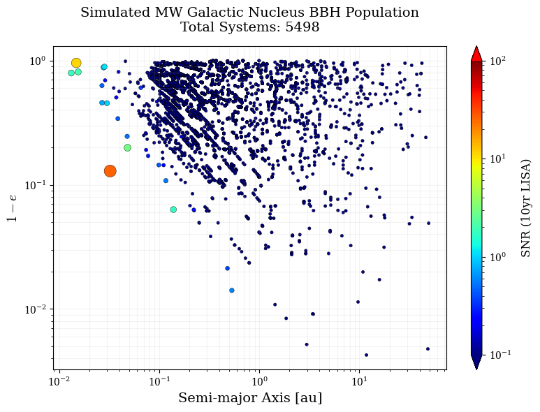
leap.GN.get_snapshot()
Generates a snapshot of the BBH population currently in the GN. This includes systems from both the steady-state formation channel and a recent starburst event (Young Nuclear Cluster, YNC). The results can be changed by adjusting the BBH formation rate in the steady-state population and the age / total BBH number in the YNC population.
- Input:
rate_gn(float, optional): Merger rate for the steady-state channel [Myr$^{-1}$]. Default2.0.age_ync(float, optional): Age of the Young Nuclear Cluster [yr]. Default6.0e6.n_ync_sys(int, optional): Number of systems to simulate for the YNC channel. Default100.max_bh_mass(float, optional): Maximum BH mass to consider [$M_\odot$]. Default50.plot(bool, optional): IfTrue, plots the snapshot population ($1-e$ vs. $a$, color-coded by SNR).
- Output:
- A list of
CompactBinaryobjects representing the BBHs currently in the Milky Way center, sorted by SNR (high to low). Each object stores the current inclination inextra['inclination_rad']and the instantaneous SNR inextra['snr'].
- A list of
Example:
gn_snapshot = leap.GN.get_snapshot(
    rate_gn=3.0, age_ync=6.0e6, n_ync_sys=100, max_bh_mass=100.0, plot=True
)
print(f"   Output List Length: {len(gn_snapshot)} systems")
- Output:
Output List Length: 5498 systems
3.2 Globular Clusters (GC)
This module models Binary Black Holes formed dynamically in Milky Way globular clusters. It supports sampling from specific dynamical formation channels (e.g., Kozai–Lidov triples, binary–single captures) based on detailed Monte Carlo N-body simulations.
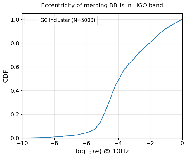
leap.GC.sample_eccentricities()
Randomly samples $N$ merger eccentricities for GC BBHs at the LIGO frequency band (10 Hz).
- Input:
n(int): Number of eccentricity samples to generate.channel_name(str, optional): Specific formation channel. Default'Incluster'.'Incluster': Weighted average of all in-cluster channels.'Ejected': Mergers occurring after ejection.- Sub-channels: Supports specific dynamical channels such as
'KL Triple','Non-KL Triple','Single Capture','Fewbody Capture'.
plot(bool, optional): IfTrue, plots the CDF of $\log_{10}(e)$.
- Output:
gc_e_samples(NumPy array): 1D array of sampled eccentricity values at 10 Hz.
Example:
gc_e_samples = leap.GC.sample_eccentricities(
    n=5000, channel_name='Incluster', plot=True
)
print(f"   Output Shape: {np.shape(gc_e_samples)}")
- Output:
Output Shape: (5000,)
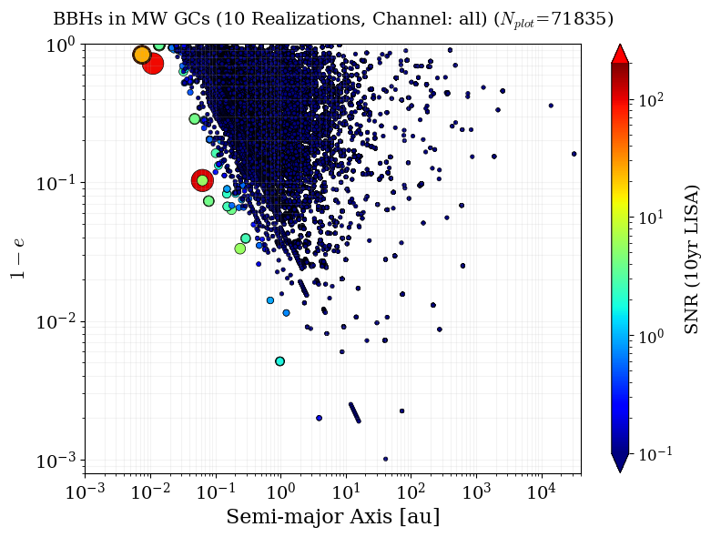
leap.GC.get_snapshot()
Retrieves a snapshot of the GC BBH population in the Milky Way. Supports three retrieval modes to allow for different scales of analysis (full ensemble vs. single galaxy realization).
- Input:
mode(str, optional): Data selection mode. Default'10_realizations'.'10_realizations': Returns the full catalog from 10 MW realizations (~2300 systems).'single': Returns data from a single MW realization (randomly selected 1/10 subset of the full catalog, ~230 systems).'random': Returns a specified number of randomly selected systems.
n_random(int, optional): Number of systems to retrieve (only used ifmode='random'). Default500.channel(str, optional): Target population group. Default'all'.'all': Both in-cluster and ejected populations.'incluster': In-cluster only (Mock_GC_BBHs.csv).'ejected': Ejected only (Mock_GC_BBHs_ejected.csv).
plot(bool, optional): IfTrue, plots the snapshot ($1-e$ vs $a$).
- Output:
- A list of
CompactBinaryobjects. - Warning: The underlying catalog represents a finite set of simulations (~230 systems per realization). If
n_randomexceeds the size of a single realization, the returned sample will inevitably mix systems from different stochastic realizations. Due to the small sample size of the MC N-body source catalog, these samples may not be strictly statistically independent.
- A list of
Example:
gc_data_full = leap.GC.get_snapshot(mode='10_realizations', plot=True)
print(f"   Output List Length: {len(gc_data_full)}")
- Output:
Output List Length: 71835
3.3 Galactic Field (Field)
This module models Binary Black Hole mergers formed via dynamical fly-by interactions in galactic field environments. It supports simulations for both Milky Way-like (disk) galaxies and elliptical galaxies.
leap.Field.run_simulation()
Executes a Monte Carlo simulation to generate a population of fly-by mergers based on specific galactic structure and physical parameters. The results are saved to disk (inside the package's data/ directory) for subsequent analysis (sampling / snapshotting).
- Input:
galaxy_type(str, optional): Target environment.'MW'(Milky Way) or'Elliptical'. Default'MW'.- Physics parameters:
m1,m2,mp(float, optional): Masses of the binary components and perturber [$M_\odot$]. Default10,10,0.6.fbh(float, optional): Fraction of stars that are wide binary black holes. Default7.5e-4.fgw(float, optional): Gravitational wave frequency used as the reference for the eccentricity distribution (default 10 Hz = LIGO band).formation_mod(str, optional): Star formation history model ('starburst','continuous'). Default'starburst'.
- Structure parameters (MW):
n0(float, optional): Stellar number density normalization in the solar neighborhood [pc$^{-3}$]. Default0.1.rsun(float, optional): Distance from the solar system to the Galactic center [pc]. Default8000.0.Rl,h(float, optional): Galactic scale lengths (radial, vertical) [pc]. Default2600.0,1000.0.sigmav(float, optional): Velocity dispersion [m/s]. Default50000.0.age_mw(float, optional): Age of the MW galaxy [years]. Default10e9.
- Structure parameters (Elliptical):
M_gal(float, optional): Total mass of the galaxy [$M_\odot$]. Default1.0e12.Re(float, optional): Effective radius (half-light radius) [pc]. Default8000.0.distance_Mpc(float, optional): Distance to the galaxy [Mpc]. Default16.8.age_ell(float, optional): Age of the elliptical galaxy [years]. Default13e9.
- Control:
arange_log(list, optional): Range of BBH semi-major axis $\log_{10}(a/\mathrm{au})$ to sample[min, max]. Default[2, 4.5].- MW-specific:
n_sim_samples(int, optional): Total number of MC trials. Default200000.target_N(int, optional): Target number of successful mergers to accumulate. Default100000.rrange_mw(list, optional): Radial range for simulation[min, max][kpc]. Default[0.5, 15].blocknum_mw(int, optional): Number of radial bins used to discretize the simulation volume. Default29. Larger values improve resolution at higher runtime.
- Elliptical-specific:
ell_n_sim(int, optional): Total number of MC trials. Default100000.ell_target_N(int, optional): Target number of successful mergers. Default50000.rrange_ell(list, optional): Radial range for simulation[min, max][kpc]. Default[0.05, 100].blocknum_ell(int, optional): Number of radial bins. Default60.
- Output:
None. Results are saved internally to the package'sdata/directory and subsequently loaded byget_progenitor,sample_eccentricities, andget_snapshot.
Example:
leap.Field.run_simulation(
    galaxy_type='MW',
    # Physics (optional overrides)
    m1=10.0, m2=10.0, mp=0.6,
    fbh=7.5e-4, fgw=10.0,
    formation_mod='starburst',
    # Structure (optional overrides)
    n0=0.1, rsun=8000.0, Rl=2600.0, h=1000.0, sigmav=50000.0,
    # Control (optional overrides)
    n_sim_samples=200000, target_N=100000, rrange_mw=[0.5, 15]
)
print("   Status: Simulation completed and saved.")
Extension: Simulating an elliptical galaxy
The simulation engine can also model massive elliptical galaxies (e.g., M87-like) by switching galaxy_type to 'Elliptical' and adjusting the structural parameters ($M_{\rm gal}$, $R_e$).
Example:
leap.Field.run_simulation(
    galaxy_type='Elliptical',
    # Structure (massive galaxy at 16.8 Mpc)
    distance_Mpc=16.8, M_gal=1.0e12, Re=8000.0,
    # Physics (heavier BHs)
    m1=30.0, m2=30.0, mp=0.6,
    # Control (smaller run for demo)
    ell_n_sim=50000, ell_target_N=20000
)
print("   Status: Elliptical simulation saved.")
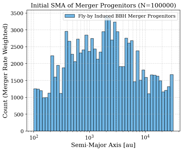
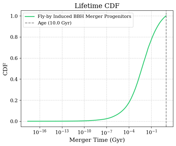
leap.Field.get_progenitor()
Retrieves the properties of the binary progenitors (initial states at formation) from the simulated library. These represent the system parameters right after being perturbed to high eccentricity and starting to evolve via GW emission.
- Input:
galaxy_type(str, optional): Target environment.'MW'or'Elliptical'. Default'MW'.plot(bool, optional): IfTrue, plots the initial semi-major axis distribution and the merger-lifetime CDF. DefaultTrue.
- Output:
- A list of
CompactBinaryobjects representing the progenitor systems. The length of the list equalstarget_N(MW) orell_target_N(Elliptical) of the precedingrun_simulationcall. - Note: These objects contain simulation statistics in their
extraattributes:merger_rate: Effective merger-rate weight for this system.lifetime_yr: Time from formation to merger.e_final_LIGO: Eccentricity when entering the LIGO band.tau_relax: Relaxation / evaporation timescale.
- A list of
Example:
field_progs = leap.Field.get_progenitor(galaxy_type='MW', plot=True)
print(f"   Output List Length: {len(field_progs)}")
- Output:
Output List Length: 100000
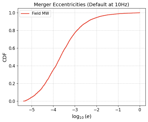
leap.Field.sample_eccentricities()
Randomly samples $N$ merger eccentricities for Field BBHs at the LIGO frequency band (10 Hz).
- Input:
n(int): Number of eccentricity samples to generate.galaxy_type(str, optional): Target environment.'MW'or'Elliptical'. Default'MW'.plot(bool, optional): IfTrue, plots the CDF of $\log_{10}(e)$.
- Output:
field_e_samples(NumPy array): 1D array of sampled eccentricity values at 10 Hz.
Example:
field_e_samples = leap.Field.sample_eccentricities(
    n=5000, galaxy_type='MW', plot=True
)
print(f"   Output Shape: {np.shape(field_e_samples)}")
- Output:
Output Shape: (5000,)
leap.Field.get_snapshot()
Generates a "snapshot" containing BBH systems currently existing in the Galactic Field. These systems represent binaries that have been excited to high eccentricity via fly-by interactions and are predicted to merge within the specified future time window (t_window_Gyr).
- Input:
mode(str, optional): Sampling mode. Default'single'.'single': One random realization based on the calculated merger rate.'multi'(MW only): Stacks multiple realizations to reduce statistical variance.'forced': Randomly selectsn_systemsregardless of physical rates (useful for testing).
galaxy_type(str, optional): Target environment. Default'MW'.t_obs(float, optional): Observation duration in years (SNR accumulation window). Default10.0.t_window_Gyr(float, optional): Future time window in which to look for merging systems.- Note: This should ideally not exceed the galaxy age (e.g., 10 Gyr). Extending the window beyond the age implies looking for systems that would likely have been removed or merged earlier in the simulation history.
n_realizations(int, optional): Number of realizations (only formode='multi'). Default10.n_systems(int, optional): Number of systems to force-sample (only formode='forced'). Default500.plot(bool, optional): IfTrue, plots the snapshot distribution. DefaultTrue.
- Output:
- A list of
CompactBinaryobjects representing the detectable sources.
- A list of
Example:
field_snapshot_mw = leap.Field.get_snapshot(
    mode='single', t_obs=10.0, t_window_Gyr=10.0, galaxy_type='MW', plot=True
)
print(f"   Output List Length: {len(field_snapshot_mw)}")
- Output:
Output List Length: 72
4️⃣ Waveform & Analysis Pipeline
This module provides a low-level functional interface to generate and analyze eccentric gravitational waveforms. It mirrors many of the CompactBinary methods but takes raw parameter inputs.
leap.Waveform.compute_waveform()
Generates the time-domain waveform ($h_+, h_\times$) using a PN evolution model.
- Input:
- Input mode selector:
input_mode(str, optional): Determines howa_auis interpreted. Default'a_au'.'a_au': Inputa_auis treated as semi-major axis [au].'forb_Hz': Inputa_auis treated as orbital frequency [Hz].'fangular_Hz': Inputa_auis treated as angular/peak frequency [Hz] (the solver finds the corresponding $f_{\rm orb}$).
a_au(float): Value corresponding toinput_mode(name kept for API stability even though the meaning switches).
- Physical parameters:
m1_msun,m2_msun(float): Component masses [$M_\odot$].e(float): Orbital eccentricity.Dl_kpc(float): Luminosity distance [kpc].tobs_yr(float): Observation duration [years].theta,phi(float, optional): Sky-position angles [rad]. Default $\pi/4$.initial_orbital_phase(float, optional): Initial mean anomaly [rad]. Default0.
- Model & sampling:
PN_orbit,PN_reaction(int, optional): Post-Newtonian orders. Default3,2.points_per_peak(int, optional): Adaptive sampling density per periastron. Default50.ts(float, optional): Fixed time step [seconds]. If set, overrides adaptive sampling.max_memory_GB(float, optional): Array-size safety limit. Default16.0.
plot(bool, optional): IfTrue, plots the waveform.
- Input mode selector:
- Output:
- A list of three NumPy arrays:
[time_vector, h_plus, h_cross].
- A list of three NumPy arrays:
Example:
# Shift specific initial phase to show periastron GW burst
e_val = 0.99
init_phase = -5*np.pi * np.power(1 - e_val, 1.5)

waveform_data = leap.Waveform.compute_waveform(
    # --- System params ---
    m1_msun=10.0, m2_msun=10.0,
    a_au=0.1, e=e_val,          # input_mode='a_au' (default): a = 0.1 AU
    Dl_kpc=8.0,
    input_mode='a_au',
    tobs_yr=0.5,
    initial_orbital_phase=init_phase,
    theta=np.pi/4, phi=np.pi/4,
    PN_orbit=3, PN_reaction=2,
    points_per_peak=50,         # adaptive sampling resolution
    plot=True, verbose=True
)

waveform_data_B = leap.Waveform.compute_waveform(
    m1_msun=10.0, m2_msun=10.0,
    a_au=1e-5, e=0.7,           # input_mode='forb_Hz': value is f_orb = 1e-5 Hz
    Dl_kpc=8.0, tobs_yr=0.1,
    input_mode='forb_Hz', ts=10, # ts disables adaptive sampling; fix dt = 10 s
    plot=False
)
- Output:
Data inspection & visualization
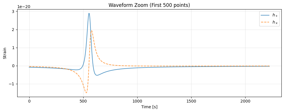
After generation, it's useful to verify the data structure, calculate the sampling interval ($\Delta t$), and visualize the waveform details (e.g., the bursty structure at periastron).
- Key step: calculate
dtfrom the first two time points (t[1] - t[0]) when using fixedts, or confirm the adaptive cadence. - Visualization: Plotting a subset (e.g., first 500 points) allows for a quick check of the polarization phases.
Example:
import matplotlib.pyplot as plt
t_vec, h_plus, h_cross = waveform_data[0], waveform_data[1], waveform_data[2]

print(f"   Output Structure: List of 3 Numpy Arrays")
print(f"      t_vec shape : {t_vec.shape}")
print(f"      h_plus shape: {h_plus.shape}")
print(f"      h_cross shape: {h_cross.shape}")

# CRITICAL: Calculate Sampling Interval (dt) for next steps
dt_val_sec = t_vec[1] - t_vec[0]
print(f"   Sample time dt    : {dt_val_sec:.4e} seconds (Passed to next step)")

# Plot first 500 points to see the burst structure
plt.figure(figsize=(10, 4))
N_plot = 500
plt.plot(t_vec[:N_plot], h_plus[:N_plot], label=r'$h_+$', alpha=0.8)
plt.plot(t_vec[:N_plot], h_cross[:N_plot], label=r'$h_\times$', alpha=0.8, ls='--')
plt.xlabel('Time [s]')
plt.ylabel('Strain')
plt.title(f'Waveform Zoom (First {N_plot} points)')
plt.legend()
plt.grid(True, alpha=0.3)
plt.tight_layout()
plt.show()
- Output:
Output Structure: List of 3 Numpy Arrays
t_vec shape : (3535099,)
h_plus shape: (3535099,)
h_cross shape: (3535099,)
Sample time dt    : 4.4604e+00 seconds (Passed to next step)
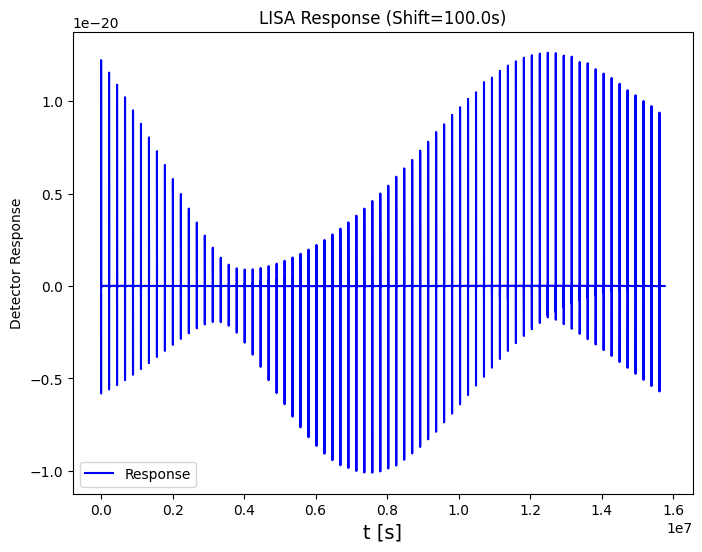
leap.Waveform.compute_LISA_response()
Computes the Time-Delay-Interferometry (TDI) response (specifically the $X$ channel / Michelson-equivalent response) for the LISA constellation. This function projects $h_+$ and $h_\times$ onto the detector arms, accounting for the antenna pattern and time delays.
- Input:
dt_sample_sec(float): Sampling interval of the input waveform [s].hplus,hcross(NumPy arrays): Input waveform polarizations (must have equal length).- Source location (ecliptic coordinates):
theta_sky(float, optional): Polar angle (co-latitude) of the source [rad]. Default $\pi/4$.phi_sky(float, optional): Azimuthal angle [rad]. Default $\pi/4$.
psi_sky(float, optional): Polarization rotation angle [rad]. Default $\pi/4$.timeshift_sec(float, optional): Initial time shift applied to the signal [s] (e.g., propagation delay). Default0.0.kappa,lamb(float, optional): Initial orbital / phase parameters for the LISA constellation. Default0.0.mode(str, optional): Output time-axis mode.'interp'(default): Output time axis matches the inputt_src; resampled and zero-padded outside the valid range.'raw': Outputs the true detector-arrival time axis (non-uniform, includes Doppler effects). No interpolation.
plot(bool, optional): IfTrue, plots the detector response.
- Output:
- A list of two NumPy arrays:
[time_vector, response_signal].
- A list of two NumPy arrays:
Example:
lisa_resp = leap.Waveform.compute_LISA_response(
    dt_sample_sec=dt_val_sec,
    hplus=h_plus,
    hcross=h_cross,
    theta_sky=1.0, phi_sky=2.0, psi_sky=0.5,
    timeshift_sec=100.0,
    plot=True
)

if lisa_resp is not None:
    t_resp, y_resp = lisa_resp[0], lisa_resp[1]
    print(f"   Output Structure: List of 2 Arrays (Time, Response)")
    print(f"   Max Response Amplitude: {np.max(np.abs(y_resp)):.4e}")
- Output:
Output Structure: List of 2 Arrays (Time, Response)
Max Response Amplitude: 1.2626e-20
leap.Waveform.compute_snr_analytical()
Sky-averaged analytical SNR. Supports a fast geometric approximation (for high-e, slowly evolving systems) and the original full-harmonic integration. It incorporates the time-evolving integration for systems that chirp significantly during the observation.
- Input:
m1_msun,m2_msun(float): Component masses [$M_\odot$].a_au(float): Semi-major axis [au].e(float): Eccentricity.Dl_kpc(float): Luminosity distance [kpc].tobs_yr(float): Observation time [years].quick_analytical(bool, optional): IfTrue, use the fast geometric approximation instead of full harmonic integration. DefaultFalse.force_evolve(bool, optional): Force the use of the time-evolving SNR integration regardless of the merger timescale. Only effective whenquick_analytical=False. DefaultFalse.evolve_threshold(float, optional): Threshold ratio that triggers the time-evolving integration automatically. Whent_merger < evolve_threshold * tobs, the system is considered to be evolving significantly during the observation and the evolving integral is used instead of the static-source one. Only effective whenquick_analytical=False. Default10.0.n_segments(int, optional): Number of log-spaced time segments used by the evolving SNR integral. Segments are denser near merger where orbital evolution is fastest. Default100.f_orb_max_Hz(float, optional): Orbital-frequency upper cutoff [Hz]. The evolving integration stops once $f_{\rm orb}$ exceeds this value, since by then the source has left the LISA band and further SNR contributions are negligible. Default0.1.verbose(bool, optional): Controls standard output printing. Default isTrue.
- Output:
snr(float): Estimated SNR value.
- Notes:
- Branch selection (when
quick_analytical=False):- If
force_evolve=True, ORt_merger < evolve_threshold * tobs, the function uses the time-evolving integral: the orbit is propagated via Peters (1964) equations along $N$ log-spaced segments from $t=0$ to $\min(t_{\rm obs}, t_{\rm merger})$, each segment contributes $d{\rm SNR}^2$ assuming the midpoint orbital parameters are static, and the total is $\sqrt{\sum d{\rm SNR}^2}$. - Otherwise (slow-evolution regime), the function falls back to the original static-source full-harmonic integration (
PN_waveform.SNR), which assumes the orbit is essentially frozen during $t_{\rm obs}$.
- If
- The evolving branch automatically truncates the integration once the orbital frequency exceeds
f_orb_max_Hz(default 0.1 Hz). This avoids numerical issues very close to merger and costs no SNR (the band is already gone).
- Branch selection (when
Example:
# Default: full integration, auto-switches to evolving if t_merger < 10 * tobs
snr_ana = leap.Waveform.compute_snr_analytical(
    m1_msun=10.0, m2_msun=10.0,
    a_au=0.1, e=0.99,
    Dl_kpc=8.0, tobs_yr=0.5,
)
print(f"   [Analytical] SNR ~ {snr_ana:.4f}")

# Force time-evolving integration with higher resolution
snr_evolve = leap.Waveform.compute_snr_analytical(
    m1_msun=10.0, m2_msun=10.0,
    a_au=0.1, e=0.99,
    Dl_kpc=8.0, tobs_yr=0.5,
    force_evolve=True, n_segments=500,
)
- Output:
[Analytical] SNR ~ 354.9420
leap.Waveform.compute_snr_numerical()
Computes SNR directly from the time-domain waveform array. Valid for arbitrary signals.
- Input:
dt_sample_sec(float): Sampling interval [s].strainlist(NumPy array): Waveform array (e.g.,h_plusor the detector response).
- Output:
snr(float): Calculated SNR value.
Example:
snr_num = leap.Waveform.compute_snr_numerical(
    dt_sample_sec=dt_val_sec,
    strainlist=h_plus
)
print(f"   [Numerical]  SNR for hplus ~ {snr_num:.4f}")
- Output:
[Numerical] SNR for hplus ~ 141.5342
leap.Waveform.compute_inner_product()
Computes the noise-weighted inner product $\langle h_1 | h_2 \rangle$ between two time-domain waveforms using the LISA sensitivity curve $S_n(f)$. This is the fundamental operation for matched filtering, overlap calculations, and determining signal orthogonality.
$$\langle h_1 | h_2 \rangle = 4 ,\mathrm{Re} \int_{f_{\min}}^{f_{\max}} \frac{\tilde{h}_1^*(f), \tilde{h}_2(f)}{S_n(f)}, df$$
- Input:
dt_sample_sec(float): Sampling interval [s].h1,h2(NumPy arrays): Time-domain signal arrays (must have the same length).phase_difference(float, optional): Relative phase shift applied during the inner product [rad]. Default0.
- Output:
inner_prod(float): The calculated inner product value.
Example:
inner_prod = leap.Waveform.compute_inner_product(
    dt_sample_sec=dt_val_sec,
    h1=h_plus,
    h2=h_plus
)
print(f"   Inner Product Value: {inner_prod:.4e}")
print(f"   Sqrt(Inner Product): {np.sqrt(inner_prod):.4f} (Should match Numerical SNR)")
- Output:
Inner Product Value: 2.0032e+04
Sqrt(Inner Product): 141.5342 (Should match Numerical SNR)
leap.Waveform.compute_merger_time()
- Input:
m1_msun,m2_msun(float): Component masses [$M_\odot$].a0_au(float): Initial semi-major axis [au].e0(float): Initial eccentricity.
- Output:
t_merge(float): Time to merger in years. Returnsinfif the system is effectively stable or parameters are invalid.
Example:
t_merge = leap.Waveform.compute_merger_time(
    m1_msun=10.0, m2_msun=10.0,
    a0_au=0.1, e0=0.99
)
print(f"   Merger Time: {t_merge:.4e} yr")
- Output:
Merger Time: 2.6811e+04 yr
leap.Waveform.evolve_orbit()
- Input:
m1_msun,m2_msun(float): Component masses [$M_\odot$].a0_au(float): Initial semi-major axis [au].e0(float): Initial eccentricity.delta_t_yr(float): Time duration to evolve forward [years]. Supports negative values for inverse evolution.
- Output:
(a_new, e_new)tuple:a_new(float): Evolved semi-major axis [au].e_new(float): Evolved eccentricity.
Example:
dt_evol = t_merge / 2.0
print(f"   Evolving forward by {dt_evol:.2e} yr...")

a_ev, e_ev = leap.Waveform.evolve_orbit(
    m1_msun=10.0, m2_msun=10.0,
    a0_au=0.1, e0=0.99,
    delta_t_yr=dt_evol
)
print(f"   Result: a={a_ev:.4e} AU, e={e_ev:.6f}")
- Output:
Evolving forward by 1.34e+04 yr...
Result: a=3.4600e-02 AU, e=0.971288
leap.Waveform.compute_characteristic_strain_single()
Computes the characteristic strain spectrum ($h_c$) for a single eccentric binary system. Provides different physically equivalent representations of the characteristic strain; see Appendix A.2 and A.3 of Xuan et al. (2026) for details.
Note: This fast method assumes the binary's evolution is negligible during the observation.
-
Input:
m1_msun,m2_msun(float): Component masses [$M_\odot$].a_au(float): Semi-major axis [au].e(float): Eccentricity.Dl_kpc(float): Luminosity distance [kpc].tobs_yr(float): Integration time [years].plot(bool, optional): IfTrue, generates a spectrum plot against the LISA sensitivity curve.
-
Output:
- A list of 5 NumPy arrays:
[freq, hc_spectrum, hc_harmonics, hc_non_evolve, snr_contrib](see the definitions in.compute_characteristic_strain()above — the output format is identical).
- A list of 5 NumPy arrays:
Example:
hc_res = leap.Waveform.compute_characteristic_strain_single(
    m1_msun=10.0, m2_msun=10.0,
    a_au=0.1, e=0.99, Dl_kpc=8.0,
    tobs_yr=0.5, plot=True
)

if isinstance(hc_res, list) and len(hc_res) == 5:
    print(f"   Output: List of 5 Elements")
    print(f"      [0] Frequency List                           (shape: {hc_res[0].shape})")
    print(f"      [1] Smoothed Spectrum (hc_env)               (shape: {hc_res[1].shape})")
    print(f"      [2] Individual Harmonics (hc_insp)           (shape: {hc_res[2].shape})")
    print(f"      [3] Non-evolving Harmonics (hc_nonevolve)    (shape: {hc_res[3].shape})")
    print(f"      [4] Contribution to Snf                      (shape: {hc_res[4].shape})")
- Output:
  Output: List of 5 Elements
     [0] Frequency List                           (shape: (14093,))
     [1] Smoothed Spectrum (hc_env)               (shape: (14093,))
     [2] Individual Harmonics (hc_insp)           (shape: (14093,))
     [3] Non-evolving Harmonics (hc_nonevolve)    (shape: (14093,))
     [4] Contribution to Snf                      (shape: (14093,))
leap.Waveform.compute_characteristic_strain_numerical()
Computes the numerical spectrum representation ($h_{c, \mathrm{num}}$) directly from a time-domain waveform array using FFT. Universally valid for any time-domain signal.
-
Formula (Ref: Appendix A.3 of Xuan et al. 2026): $$h_{c, \mathrm{num}}[k] = \sqrt{\frac{2 f_k}{T_{\mathrm{obs}}}}; |\tilde{h}(f_k)|$$
Physics note: In the non-evolving limit ($\dot{f} \to 0$), the comb-like peak heights of this numerical spectrum coincide with the discrete harmonic representation ($h_{c, \mathrm{non\text{-}evolve}}$). They will appear lower than the smoothed envelope ($h_{c, \mathrm{env}}$) by a factor of $\sqrt{f_{\mathrm{orb}}/f}$, as the smoothed envelope redistributes energy to preserve the integrated SNR.
-
Input:
h_t(NumPy array or list): Time-domain waveform strain sequence (e.g., $h_+$ or detector response).ts(float): Sampling rate in Hz (i.e.,1 / dt).plot(bool, optional): IfTrue, plots the numerical characteristic strain spectrum against the LISA sensitivity curve.
-
Output:
- A
tupleof two NumPy arrays:(xs, hc_num).[0] xs: Frequency axis [Hz] (positive half-space).[1] hc_num: Numerical characteristic strain spectrum ($h_{c, \mathrm{num}}$).
- A
Example:
# Assuming 'h_plus' and 'dt_val_sec' are available from a previous waveform computation
f_num, hc_num = leap.Waveform.compute_characteristic_strain_numerical(
    h_t=h_plus,
    ts=1.0 / dt_val_sec,
    plot=True
)

print(f"   Output: Tuple of 2 Elements")
print(f"      [0] Frequency Axis     (shape: {f_num.shape})")
print(f"      [1] Numerical Spectrum (shape: {hc_num.shape})")
- Output:
   Output: Tuple of 2 Elements
      [0] Frequency Axis     (shape: (1767549,))
      [1] Numerical Spectrum (shape: (1767549,))
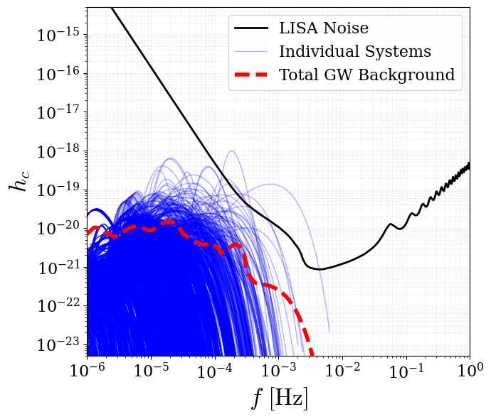
leap.Waveform.run_population_strain_analysis()
Performs a batch characteristic strain analysis on a population of binaries. Iterates through a list of CompactBinary objects, computes their individual spectra, and aggregates the results to estimate the total signal background or confusion noise.
- Input:
binary_list(list): A list ofCompactBinaryobjects (e.g., fromGC.get_snapshot()orField.get_snapshot()).tobs_yr(float): Integration time [years].plot(bool, optional): IfTrue, plots the combined population spectrum against the LISA sensitivity curve.
- Output:
- A
listof aggregated results:faxis: Common frequency axis array.Snf_tot: Total noise PSD contribution from the population.all_fn_lists: List of per-binary frequency arrays.all_hcavg_lists: List of per-binary time-integrated $h_c$ arrays.all_hnc_lists: List of per-binary instantaneous $h_c$ arrays.
- A
Example:
if 'gn_snapshot' in locals() and len(gn_snapshot) > 0:
    batch_res = leap.Waveform.run_population_strain_analysis(
        binary_list=gn_snapshot,
        tobs_yr=4.0,
        plot=True
    )

    if batch_res is not None:
        faxis, Snf_tot = batch_res[0], batch_res[1]
        print(f"   Output Structure: [faxis, Snf_tot, ...]")
        print(f"      faxis shape  : {faxis.shape}")
        print(f"      Snf_tot shape: {Snf_tot.shape}")
else:
    print("   [Skip] No population snapshot available for batch analysis.")
- Output:
Output Structure: [faxis, Snf_tot, ...]
  faxis shape  : (1000,)
  Snf_tot shape: (1000,)
5️⃣ Noise Management
This module lets users customize the LISA sensitivity curve used across the package. It supports generating specific noise models (e.g., N2A5 with galactic foregrounds) and inspecting them as characteristic strain.
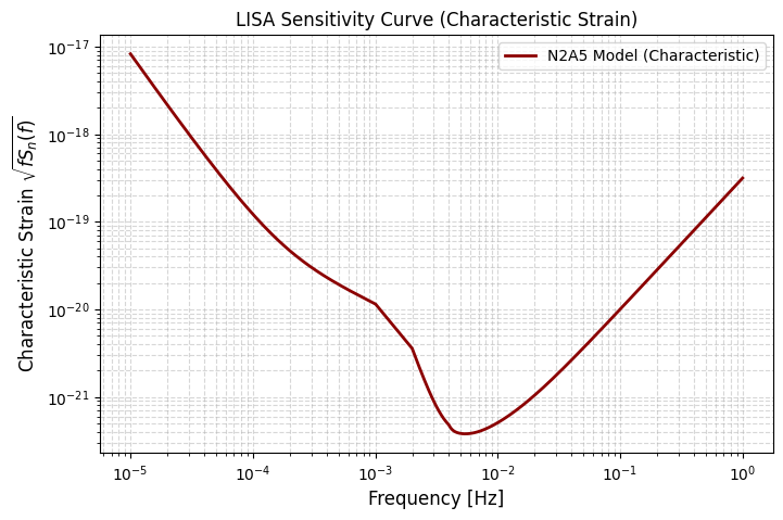
leap.Noise.generate_noise_data()
Generates synthetic noise amplitude-spectral-density (ASD) data on a specified frequency grid.
- Input:
model(str, optional): Noise model. Default'N2A5'.'N2A5': Analytical LISA sensitivity including a specific realization of the galactic confusion-noise foreground.'official': Loads a tabulated ASD fromLISA_noise_ASD_official.csvinside the package directory and interpolates (log-log, with power-law extrapolation below the tabulated range). Returns zeros if the file is missing.
f_min,f_max(float, optional): Frequency bounds [Hz]. Default1e-6,1.0.n_points(int, optional): Number of log-spaced frequency points. Default3000.
- Output:
f_new(NumPy array): Frequency grid [Hz].asd_new(NumPy array): ASD [Hz$^{-1/2}$].
Example:
f_new, asd_new = leap.Noise.generate_noise_data(
    model='N2A5', f_min=1e-5, f_max=1.0
)
print(f"   Generated Data: {len(f_new)} points.")
print(f"   Freq Range: [{f_new[0]:.1e}, {f_new[-1]:.1e}] Hz")
noise_char_strain = asd_new * np.sqrt(f_new)
# Plotting Characteristic Strain
plt.figure(figsize=(8, 5))
plt.loglog(f_new, noise_char_strain, label='N2A5 Model (Characteristic)',
           color='darkred', linewidth=2)
plt.title("LISA Sensitivity Curve (Characteristic Strain)")
plt.xlabel("Frequency [Hz]", fontsize=12)
plt.ylabel(r"Characteristic Strain $\sqrt{f S_n(f)}$", fontsize=12)
plt.grid(True, which='both', linestyle='--', alpha=0.5)
plt.legend()
plt.show()
- Output:
Generated Data: 3000 points.
Freq Range: [1.0e-05, 1.0e+00] Hz
leap.Noise.update_noise_curve()
Overwrites the on-disk noise file (LISA_noise_ASD.csv) and re-injects the new curve into the downstream waveform/SNR modules. The previous curve is automatically backed up (with incrementing indices _1, _2, …).
- Input:
data(list):[frequency_array, asd_array].
Example:
# Inject the new noise curve into the global system
leap.Noise.update_noise_curve([f_new, asd_new])
leap.Noise.recover_noise_curve()
Reverts the noise configuration to a previous backup or a standard preset.
- Input:
version(int or str):int(e.g.,1): Reverts to a specific backup (e.g.,LISA_noise_ASD_original_1.csv).'official': Reverts to the shipped official LISA sensitivity curve (LISA_noise_ASD_official.csv).'N2A5': Reverts toLISA_noise_ASD_N2A5.csv.None: Reverts to the most recent backup (_1).
Example:
leap.Noise.recover_noise_curve(version=1)
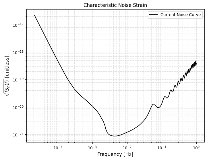
leap.Noise.get_noise_curve()
Retrieves the currently active noise data for inspection.
- Input:
plot(bool, optional): IfTrue, plots the current characteristic strain $\sqrt{f S_n(f)}$.
- Output:
- A list
[frequency_array, characteristic_strain_array], orNoneif the file cannot be read.
- A list
Example:
curve_data = leap.Noise.get_noise_curve(plot=True)
- Output:
leap.Noise.clean_backups()
Removes all temporary noise backup files (LISA_noise_ASD_original_*.csv) created during the session.
Example:
leap.Noise.clean_backups()


Download files
Download the file for your platform. If you're not sure which to choose, learn more about installing packages.
Source Distribution
Built Distribution
Filter files by name, interpreter, ABI, and platform.
If you're not sure about the file name format, learn more about wheel file names.
Copy a direct link to the current filters
File details
Details for the file lisa_leap-0.1.3.tar.gz.
File metadata
- Download URL: lisa_leap-0.1.3.tar.gz
- Upload date:
- Size: 36.2 MB
- Tags: Source
- Uploaded using Trusted Publishing? No
- Uploaded via: twine/6.2.0 CPython/3.12.9
File hashes
| Algorithm | Hash digest | |
|---|---|---|
| SHA256 |
5868f67041c63a8b1c0ede091ade061e029f69e494eee7e8ad9e839eb01fb25e
|
|
| MD5 |
86e3e3cf9a3f3a1c09a894abdb462d8c
|
|
| BLAKE2b-256 |
05ac26a491a7631687f09c07afb958bf3767e78fd122e68ab5e5471a5ef52af4
|
File details
Details for the file lisa_leap-0.1.3-py3-none-any.whl.
File metadata
- Download URL: lisa_leap-0.1.3-py3-none-any.whl
- Upload date:
- Size: 36.1 MB
- Tags: Python 3
- Uploaded using Trusted Publishing? No
- Uploaded via: twine/6.2.0 CPython/3.12.9
File hashes
| Algorithm | Hash digest | |
|---|---|---|
| SHA256 |
4ff60775e174b0a941027f24f83214bbca28308c61dfbb1d24d9bab818ab7a2e
|
|
| MD5 |
262f003c56f3433028de97258904eac1
|
|
| BLAKE2b-256 |
15ac43423206a7f728bb13fed70a6da3803eaceb187c7b0128c64e3218ce6f19
|


