
LIVE PLOT LIBrary (liveplotlib)
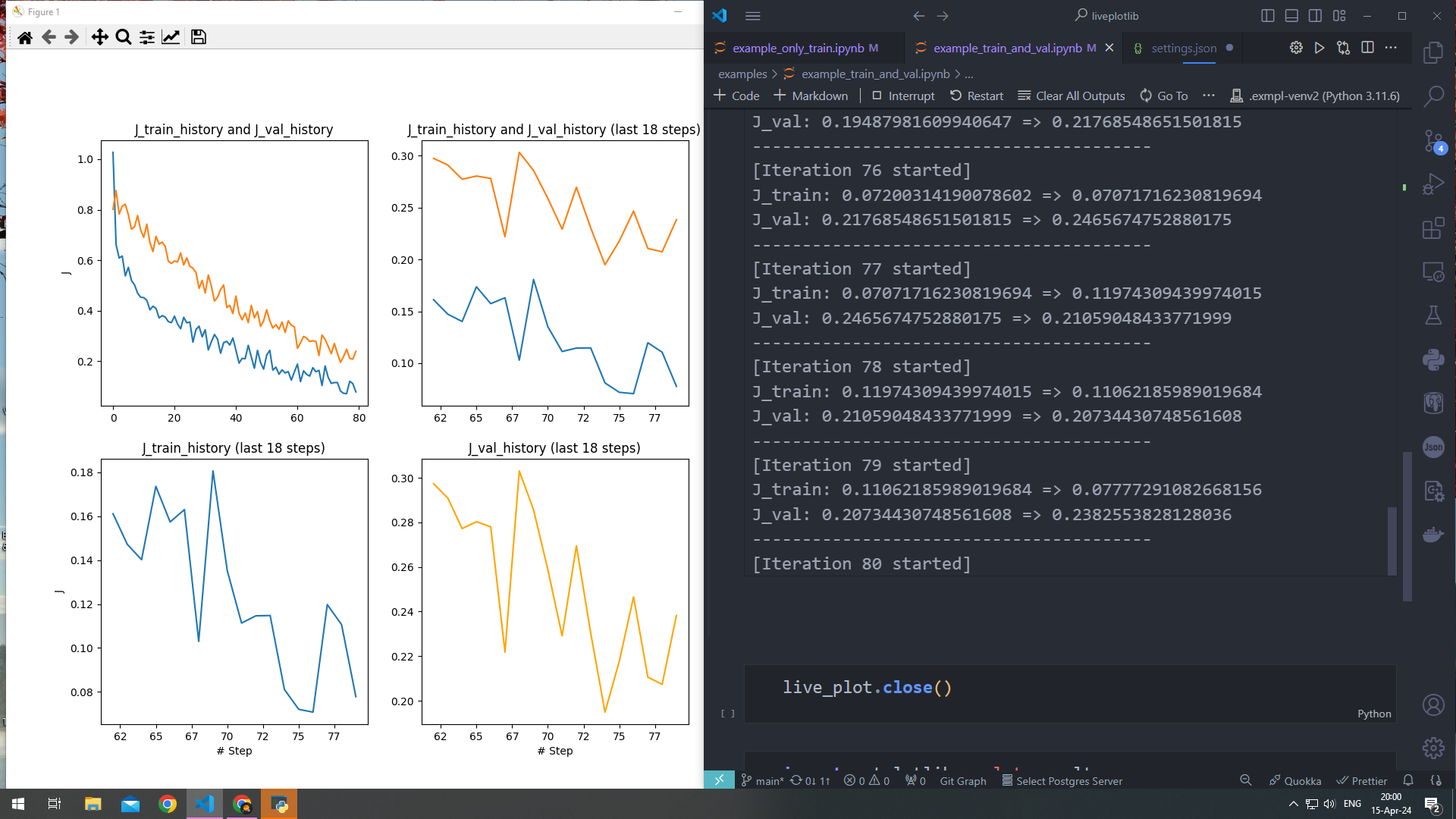
- Library for plotting (visualizing) cost function changes during model training (in real time)
- please, check compatibility to see if this library meets your needs and environment
Notations
Specific
-
J- cost/loss function
It measures how well does your model performs and used for optimization of your model -
J_history- python list (of numbers), that contains previous values of J
(for example, in previous epochs)
For subsets
J_train_history- J_history, where J was calculated on train subsetJ_val_history- J_history, where J was calculated on val subsetJ_test_history- J_history, where J was calculated on test subset
General
-
plotting- visualizing, making graph -
train/val/test- subsets of your original dataset -
train- train subset.
Used for optimizing the model parameters (weights and biases) -
val/valid- validation subset
(aka Cross-Validation (cv) or DEVeleopment (dev) subset). Used for optimizing the hyperparameters of your model (for example: learning_rate or regularization term) -
test- test subset, used for testing how your model performs on new data -
epoch- 1 iteration through the whole dataset (or subset).
Installation
>> pip install liveplotlib
# all dependencies will be installed automatically
Usage
-
Only 5 steps!
-
"foo" in names means "this is just for example, it means nothing"
-
Basic functionality:
from liveplotlib import LivePlotOnlyTrain

J_train_history = []

# begin session
live_plot = LivePlotOnlyTrain()

# update during training
# J_train_history.append(new_J_train)
live_plot.update(J_train_history)

# end session
live_plot.close()

# (See explanations below)
Option 1: plot only J_train_history
# STEP 1: IMPORT

from liveplotlib import LivePlotOnlyTrain


# ...............
# Some operations with data
# ................


# STEP 2: CREATE HISTORY LIST

# Along with model initialization, create empty J_train_history as well
model = FooSomeModelClass()
J_train_history = []


# STEP 3: INITIALIZE LIVE PLOT

# Right before training
live_plot = LivePlotOnlyTrain()


# STEP 4: UPDATE DURING TRAINING

# -----Inside train function loop-----
# ...
# new_J_train = ...
# ...
J_train_history.append(new_J_train)
# ...
live_plot.update(J_train_history)
# ...
# ------------------------------------


# STEP 5: END SESSION

# In the end (especially important in jupyter notebooks)
live_plot.close()
Option 2: plot J_train_history and J_val_history
# STEP 1: IMPORT

from liveplotlib import LivePlotTrainAndVal


# ...............
# Some operations with data
# ................


# STEP 2: CREATE HISTORY LISTS

# Along with model initialization, create empty J_train_history and J_val_history as well
model = FooSomeModelClass()
J_train_history = []
J_val_history = []


# STEP 3: INITIALIZE LIVE PLOT (START SESSION)

# Right before training
live_plot = LivePlotTrainAndVal()


# STEP 4: UPDATE DURING TRAINING

# -----Inside train function loop-----
# ...
# new_J_train = ...
# new_J_val = ...
# ...
J_train_history.append(new_J_train)
J_val_history.append(new_J_val)
# ...
live_plot.update(J_train_history, J_val_history)
# ...
# ------------------------------------


# STEP 5: END SESSION

# In the end (especially important in jupyter notebooks)
live_plot.close()
About
What does it do
- This tool
plots Cost (loss) functionchangesin real time in separated window(during training, not after its done) so you could see tendencies and diagnose/manage your optimization process more easily.
Who is it created for
- This
python libraryis created for data scientists / ML engineers / data analysts or anyone else interested
Under the hood
- written on top of matplotlib library, using its figures, subplots and lines mechanics
Compatibility
- it works only if you are running it on your local machine.
(It can't run in Google colab, because google colab's notebooks run on a remote server, so you can't exit inline mode => it will give you an error if you try).
If you have any ideas how to fix this, please, feel free to propose such important improvement )) - compatible with
.pyand.ipynb(jupyter notebook) files - It automatically determines a caller file's format and takes appropriate actions
How to
Change slice size
Slice size is calculated in each .update() by formula:
slice_size = slice_fraction * len(J_history) + slice_bias
where slice_fraction and slice_bias are parameters of .__init__() function (used for initializing live_plot).
So, if you want to add some fixed number to amount of steps to plot, increase slice_bias. If you want to make a scalable, dynamic change (like increase fraction) - then, of corse increase slice_fraction
Recomendations
If you are using LivePlotTrainAndVal
- Ensure, that your J_train_history and J_val_history have the same length.
- Update once in epoch
If you are using minibaches, then calculate J_train and J_val across all minibatches (average). Then, as always:# In the end of epoch J_train_history.append(J_train) J_val_history.append(J_val) live_plot.update(J_train_history, J_val_history)
Comments
- name "liveplotlib" comes from its "parent" library - matplotlib. (liveplotlib is written on top of matplotlib)
- please, feel free to give me feedback, propose some improvements/new functionality or report a bug.
1 maintainer

Metadata
1 maintainer
Release files for liveplotlib 0.3.3
For a detailed explanation of source distributions (sdists) and built distributions (wheels), please see the package formats documentation.
Source distribution (sdist)
| File | Size | Uploaded | |
|---|---|---|---|
| liveplotlib-0.3.3.tar.gz | 8.6 kB | Details |
Built distribution (wheel)
| File | Interpreter | ABI | Platform | Reset |
|---|---|---|---|---|
| liveplotlib-0.3.3-py3-none-any.whl | Python 3 | none | any | Details |
Total release size: 17.4 kB
Release files / liveplotlib-0.3.3.tar.gz
| Download URL | liveplotlib-0.3.3.tar.gz |
|---|---|
| Size | 8.6 kB |
| Tags | Source |
|
SHA-256 checksum How to use checksums |
09fe5f89cecf09445fb6830e181bde91c9bc2e79116ec75ce373761c8106d28c
|
|
BLAKE2b-256 checksum How to use checksums |
29c2471a5be504419ce1a904eb6f571124d1cc1f0f7acf9acdbca81f713c6b2d
|
| Upload date | |
|
Uploaded using Trusted Publishing? What is trusted publishing? |
No |
| Uploaded via |
twine/5.0.0 CPython/3.11.6
|
Release files / liveplotlib-0.3.3-py3-none-any.whl
| Download URL | liveplotlib-0.3.3-py3-none-any.whl |
|---|---|
| Size | 8.8 kB |
| Tags | Python 3 |
|
SHA-256 checksum How to use checksums |
49ea31980be92d527d44a53e1c83a3391f7754c7a8bb074ef0def525cdfcc565
|
|
BLAKE2b-256 checksum How to use checksums |
b19d13a8aef1b98bcaebc27d7791d52df48daf2bd5fd983f00d05ff89490aebd
|
| Upload date | |
|
Uploaded using Trusted Publishing? What is trusted publishing? |
No |
| Uploaded via |
twine/5.0.0 CPython/3.11.6
|














