
Draw Logistic Regression Plots in Python

Project description






lorepy: Logistic Regression Plots for Python
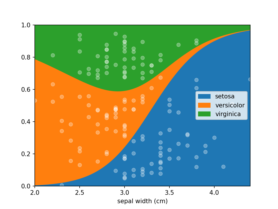
Logistic Regression plots are used to plot the distribution of a categorical dependent variable in function of a continuous independent variable.
If you prefer an R implementation of this package, have a look at loreplotr.
Why use lorepy ?
Lorepy offers distinct advantages over traditional methods like stacked bar plots. By employing a linear model, Lorepy captures overall trends across the entire feature range. It avoids arbitrary cut-offs and segmentation, enabling the visualization of uncertainty throughout the data range.
You can find examples of the Iris data visualized using stacked bar plots here for comparison.
Installation
Lorepy can be installed using pip using the command below.
pip install lorepy
Usage
Data needs to be provided as a DataFrame and the columns for the x (independent continuous) and y (dependant categorical)
variables need to be defined. Here the iris dataset is loaded and converted to an appropriate DataFrame. Once the data
is in shape it can be plotted using a single line of code loreplot(data=iris_df, x="sepal width (cm)", y="species").
from lorepy import loreplot

from sklearn.datasets import load_iris
import matplotlib.pyplot as plt
import pandas as pd

iris_obj = load_iris()
iris_df = pd.DataFrame(iris_obj.data, columns=iris_obj.feature_names)

iris_df["species"] = [iris_obj.target_names[s] for s in iris_obj.target]

loreplot(data=iris_df, x="sepal width (cm)", y="species")

plt.show()
Options
While lorepy has very few customizations, it is possible to pass arguments through to Pandas' DataFrame.plot.area and Matplotlib's pyplot.scatter to change the aesthetics of the plots.
Disable sample dots
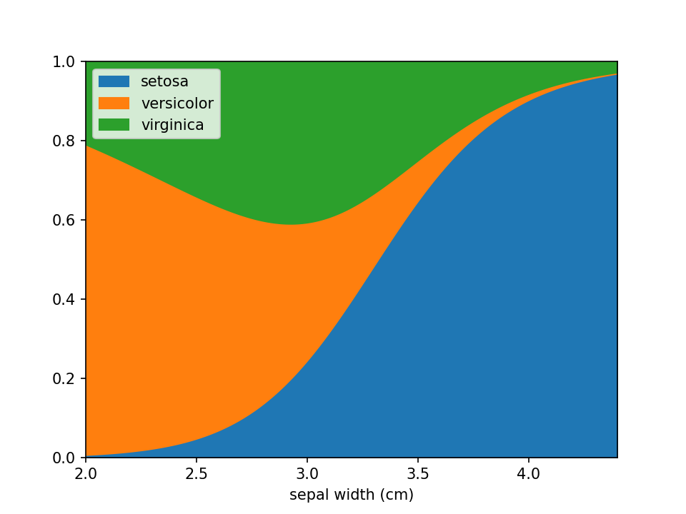
Dots indicating where samples are located can be en-/disabled using the add_dots argument.
loreplot(data=iris_df, x="sepal width (cm)", y="species", add_dots=False)
plt.show()
Custom styles
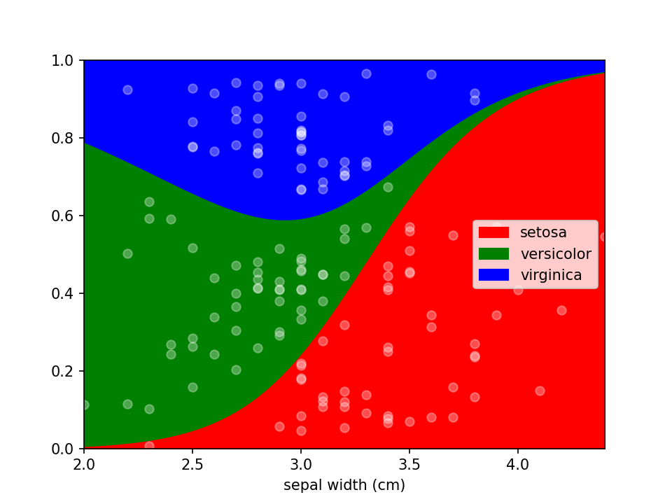
Additional keyword arguments are passed to Pandas' DataFrame.plot.area. This can be used, among other things, to define a custom colormap. For more options to customize these plots consult Pandas' documentation.
from matplotlib.colors import ListedColormap

colormap=ListedColormap(['red', 'green', 'blue'])

loreplot(data=iris_df, x="sepal width (cm)", y="species", colormap=colormap)
plt.show()
Using scatter_kws arguments for pyplot.scatter
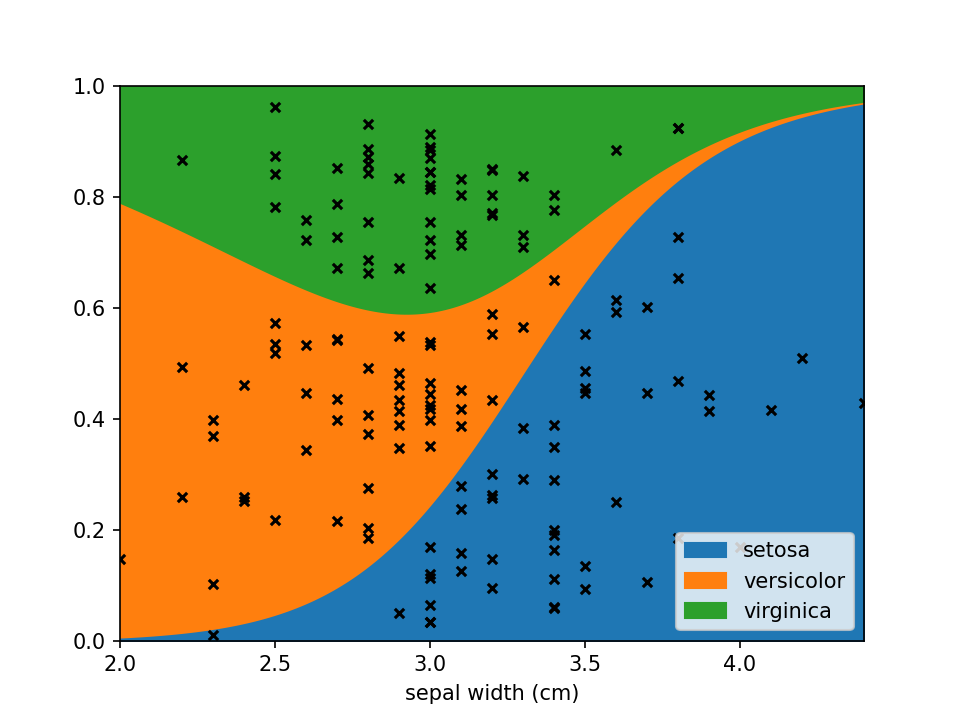
can be set to change the appearance of the sample markers.
scatter_options = {
    's': 20,                  # Marker size
    'alpha': 1,               # Fully opaque
    'color': 'black',         # Set color to black
    'marker': 'x'             # Set style to crosses
}

loreplot(data=iris_df, x="sepal width (cm)", y="species", scatter_kws=scatter_options)
plt.show()
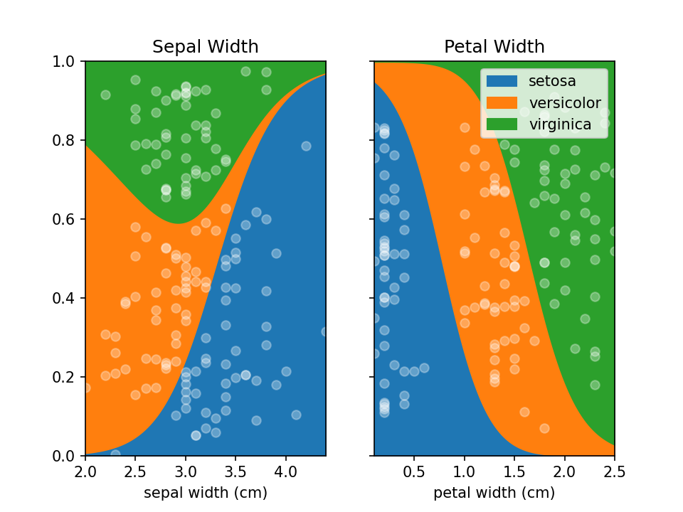
You can use LoRePlots in subplots as you would expect.
fig, ax = plt.subplots(1,2, sharex=False, sharey=True)
loreplot(data=iris_df, x="sepal width (cm)", y="species", ax=ax[0])
loreplot(data=iris_df, x="petal width (cm)", y="species", ax=ax[1])

ax[0].get_legend().remove()
ax[0].set_title("Sepal Width")
ax[1].set_title("Petal Width")

plt.savefig('./docs/img/loreplot_subplot.png', dpi=150)
plt.show()
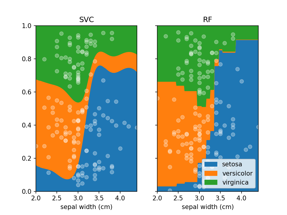
By default lorepy uses a multi-class logistic regression model, however this can be replaced with any classifier
from scikit-learn that implements predict_proba and fit. Below you can see the code and output with a
Support Vector Classifier (SVC) and Random Forest Classifier (RF).
from sklearn.svm import SVC
from sklearn.ensemble import RandomForestClassifier

fig, ax = plt.subplots(1, 2, sharex=False, sharey=True)

svc = SVC(probability=True)
rf = RandomForestClassifier(n_estimators=10, max_depth=2)

loreplot(data=iris_df, x="sepal width (cm)", y="species", clf=svc, ax=ax[0])
loreplot(data=iris_df, x="sepal width (cm)", y="species", clf=rf, ax=ax[1])

ax[0].get_legend().remove()
ax[0].set_title("SVC")
ax[1].set_title("RF")

plt.savefig("./docs/img/loreplot_other_clf.png", dpi=150)
plt.show()
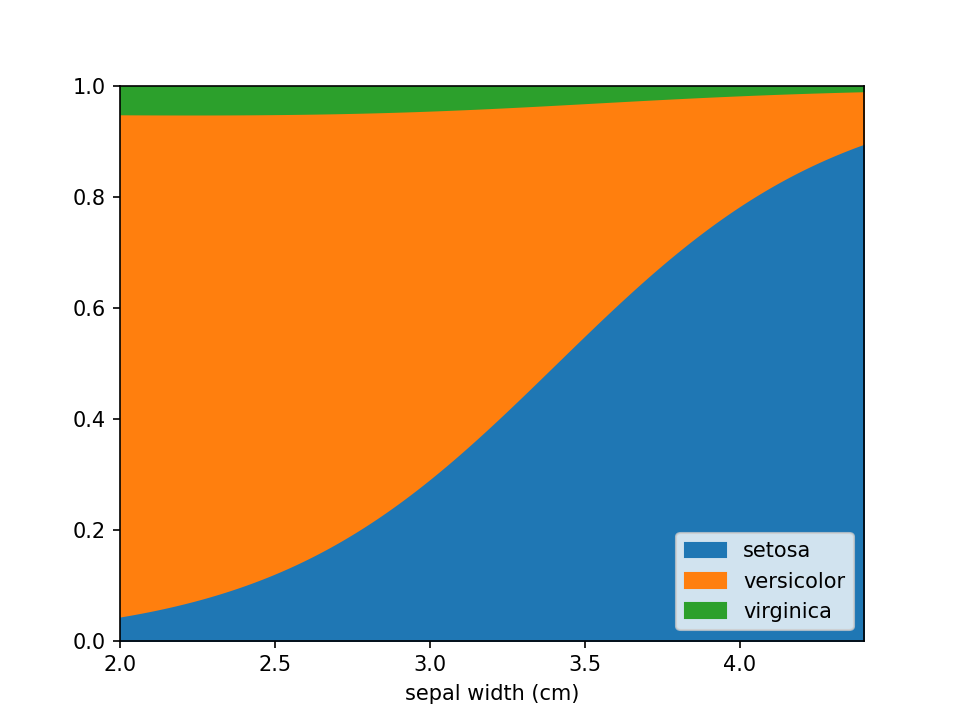
In case there are confounders, these can be taken into account using the confounders argument. This requires a
list of tuples, with the feature and the reference value for that feature to use in plots. E.g. if you wish to deconfound
for Body Mass Index (BMI) and use a BMI of 25 in plots, set this to [("BMI", 25)].
loreplot(
    data=iris_df,
    x="sepal width (cm)",
    y="species",
    confounders=[("petal width (cm)", 1)],
)
plt.savefig("./docs/img/loreplot_confounder.png", dpi=150)
plt.show()
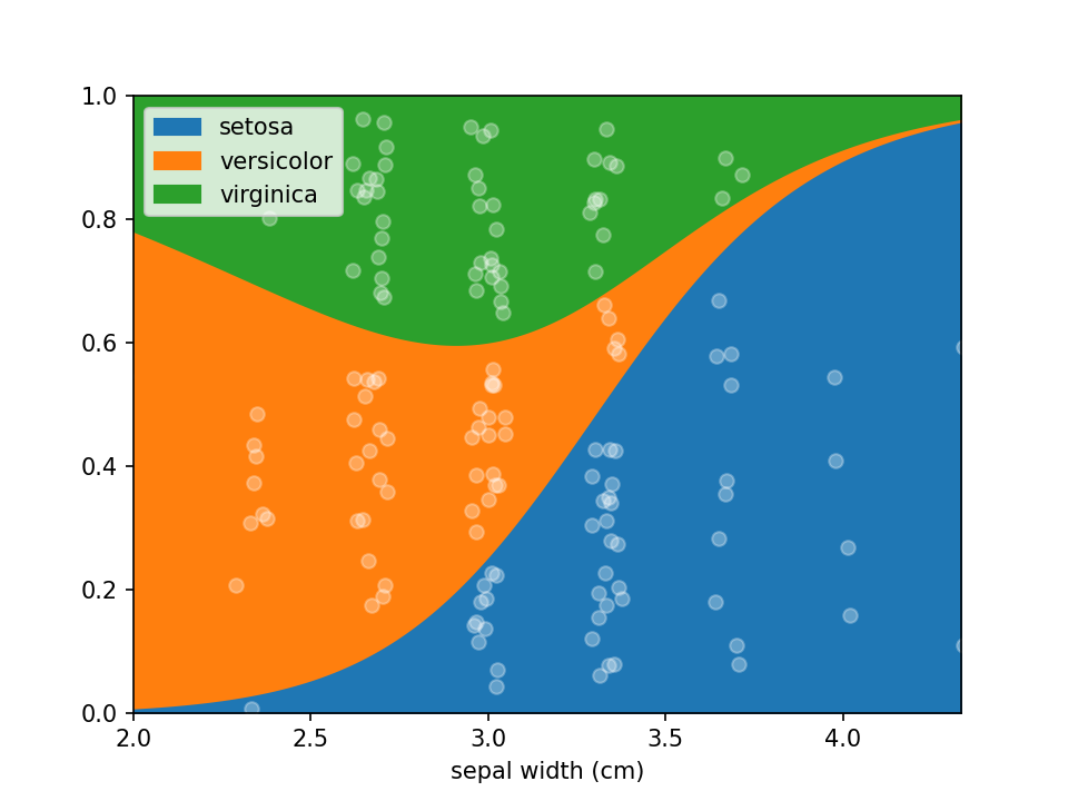
In some cases the numerical feature on the x-axis isn't continuous (e.g. an integer number), this can lead to
overplotting the dots. To avoid this to some extent a jitter feature is included, that adds some uniform noise to
the x-coordinates of the dots. The value specifies the range of the uniform noise added, the value of 0.05 in the
example sets this range to [-0.05, 0.05].
iris_df["sepal width (cm)"] = (
    np.round(iris_df["sepal width (cm)"] * 3) / 3
)  # Round values

loreplot(data=iris_df, x="sepal width (cm)", y="species", jitter=0.05)
plt.savefig("./docs/img/loreplot_jitter.png", dpi=150)
plt.show()
Assess uncertainty
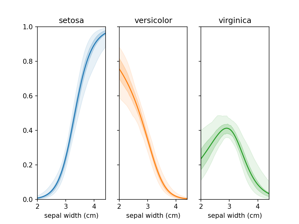
From loreplots it isn't possible to assess how certain we are of the prevalence of each group across the range. To
provide a view into this there is a function uncertainty_plot, which can be used as shown below. This will use
resampling (or jackknifing) to determine the 50% and 95% interval of predicted values and show these in a
multi-panel plot with one plot per category.
from lorepy import uncertainty_plot

uncertainty_plot(
    data=iris_df,
    x="sepal width (cm)",
    y="species",
)
plt.savefig("./docs/img/uncertainty_default.png", dpi=150)
plt.show()
This also supports custom colors, ranges and classifiers. More examples are available in example_uncertainty.py.
Development
Additional documentation for developers is included with details on running tests, building and deploying to PyPi.
Contributing
Any contributions you make are greatly appreciated.
- Found a bug or have some suggestions? Open an issue.
- Pull requests are welcome! Though open an issue first to discuss which features/changes you wish to implement.
Contact
lorepy was developed by Sebastian Proost at the RaesLab and was based on R code written by Sara Vieira-Silva. As of version 0.2.0 lorepy is available under the Creative Commons Attribution-NonCommercial-ShareAlike 4.0 International license.
For commercial access inquiries, please contact Jeroen Raes.


Download files
Download the file for your platform. If you're not sure which to choose, learn more about installing packages.
Source Distribution
Built Distribution
Filter files by name, interpreter, ABI, and platform.
If you're not sure about the file name format, learn more about wheel file names.
Copy a direct link to the current filters
File details
Details for the file lorepy-0.4.2.tar.gz.
File metadata
- Download URL: lorepy-0.4.2.tar.gz
- Upload date:
- Size: 17.8 kB
- Tags: Source
- Uploaded using Trusted Publishing? No
- Uploaded via: twine/4.0.2 CPython/3.10.0
File hashes
| Algorithm | Hash digest | |
|---|---|---|
| SHA256 |
b0a89d6bfaec82f34a2480e2accee75096d3b4d0e096db6d1a7a610754664797
|
|
| MD5 |
8a1debb694eda4df8d8548d3def3602b
|
|
| BLAKE2b-256 |
cde57b059aff1703a7341bb81c8c523d7b19b8ed7f4ae5431fa8972fca3f4b44
|
File details
Details for the file lorepy-0.4.2-py3-none-any.whl.
File metadata
- Download URL: lorepy-0.4.2-py3-none-any.whl
- Upload date:
- Size: 14.8 kB
- Tags: Python 3
- Uploaded using Trusted Publishing? No
- Uploaded via: twine/4.0.2 CPython/3.10.0
File hashes
| Algorithm | Hash digest | |
|---|---|---|
| SHA256 |
d043ad88f1ff9742600ad48c6db69354b1458c9fd79c335dd95ef0282b24be45
|
|
| MD5 |
fb3eebf6691e884b7a45db463d2e325b
|
|
| BLAKE2b-256 |
8ab92b38255fa84598cbcf5af98265f6fcce73e6358185780703f1e07a6f3bab
|






