
loss-landscape-3d (Topography Generator)


loss-landscape-3d is a lightweight, high-performance PyTorch library that samples the weight space of neural networks to generate interactive 3D visualizations of their loss landscapes.
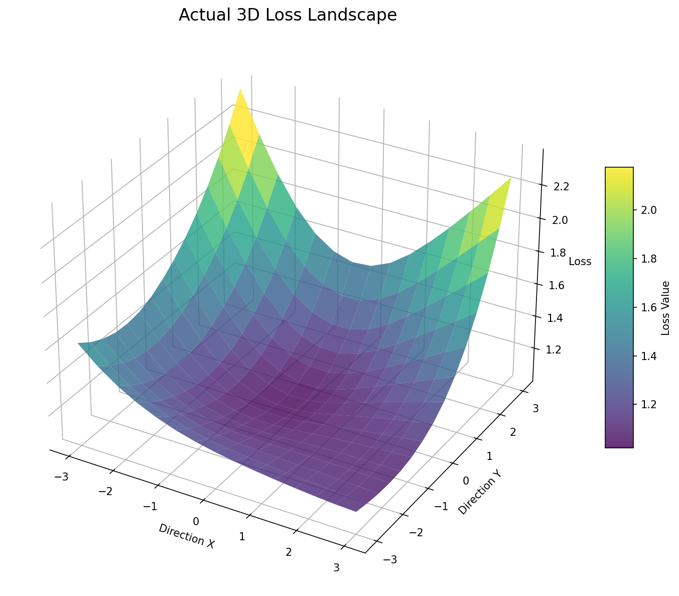
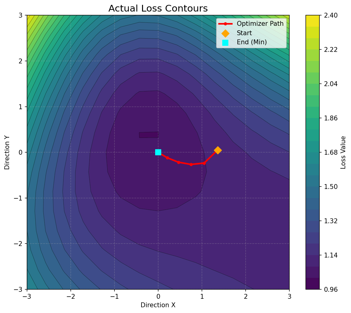
With this library, you can easily:
- Evaluate local geometry around a model's minimum using filter-wise normalization to prevent scale-invariance distortions.
- Track the exact trajectory your optimizer (e.g., SGD, Adam, RMSprop) took during training.
- Project high-dimensional optimization trajectories into a 2D coordinate system using an optimized Gram-matrix SVD method that works in seconds even for models with millions of parameters.
- Generate interactive, beautiful 3D Plotly surface charts showing the optimizer's path down the "loss mountain," highlighting concepts like local minima, saddle points, and flatness.
- Compute Hessian Eigenvector Directions (second-order curvature) to visualize the sharpest descent directions (worst-case curvature) around local minima.
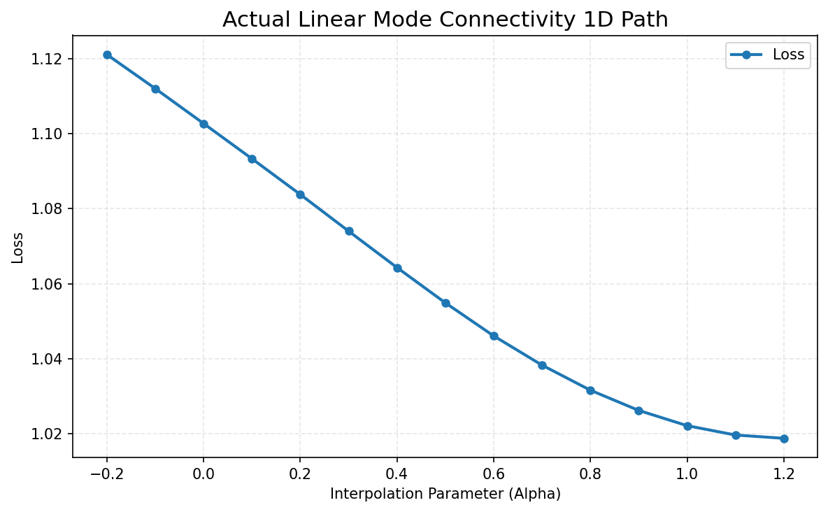
- Compute 1D Path Interpolation (Linear Mode Connectivity) to analyze the loss and accuracy barrier separating different weight states.
- Auto-detect optimal step limits using Adaptive Step Scaling to prevent manual coordinate searching.
🛠️ Installation
Install the library directly from PyPI:
pip install loss-landscape-3d
Developing Locally / Installing from Source
If you want to contribute, modify the code, or run the test suite:
git clone https://github.com/ArnavAgarwal-Mr-AR/loss-landscape-3d.git
cd loss-landscape-3d
pip install -e ".[dev]"
📐 The Mathematics Behind the Topography
1. Filter-Wise Normalization
Neural networks exhibit scale invariance (especially when using Rectified Linear Units (ReLU) and Batch Normalization). For instance, multiplying weights of one layer by a scalar $\alpha$ and dividing the next layer by $\alpha$ leaves the outputs unchanged. Without normalization, a random perturbation direction vector in parameter space will create a distorted visualization—making a model with larger weights look artificially flat and one with smaller weights look sharp.
To remove this distortion, loss-landscape-3d applies filter-wise normalization (from Li et al. "Visualizing the Loss Landscape of Neural Nets" (2018)). For each filter (or neuron row) $i$ in weight parameter $W$:
$$d_i \leftarrow d_i \cdot \frac{|W_i|_F}{|d_i|_F}$$
where $|\cdot|_F$ is the Frobenius norm. This scales the random directions proportionally to the weight magnitudes at that filter/neuron.
2. Trajectory Projection via PCA & Gram SVD
During training, a model parameter trajectory is recorded: $\theta^{(0)}, \theta^{(1)}, \dots, \theta^{(T)} \in \mathbb{R}^N$, where $N$ is the number of parameters (often millions) and $T$ is the number of checkpoints. To visualize the trajectory and the surrounding loss surface on the same plot, we must project the parameter states onto a 2D plane. We do this by finding the two directions of maximum variance using Principal Component Analysis (PCA).
Standard PCA requires computing eigenvectors of the $N \times N$ covariance matrix, which is computationally impossible when $N \approx 10^7$.
Instead, loss-landscape-3d implements an optimized SVD of the centered checkpoints matrix $X \in \mathbb{R}^{M \times N}$ ($M = T+1$):
- Compute the Gram matrix $K = X X^T \in \mathbb{R}^{M \times M}$. Since $M \ll N$ (typically $\le 100$ checkpoints), this is extremely small.
- Perform Eigendecomposition of $K$: $K = U \Lambda U^T$.
- Compute the principal components $V \in \mathbb{R}^{N \times 2}$ as $V = X^T U_2 \Sigma_2^{-1}$, where $U_2$ and $\Sigma_2$ correspond to the top 2 singular values.
- Project the checkpoints onto the plane: $\text{Coords}_t = (x_t, y_t) = (\langle \theta^{(t)} - \theta^, V_0 \rangle, \langle \theta^{(t)} - \theta^, V_1 \rangle)$, where $\theta^*$ is the center parameter (usually the final trained state).
Our implementation automatically handles rank-deficient trajectories (e.g. collinear checkpoints) by using Gram-Schmidt orthogonalization to inject a secondary independent axis when needed, ensuring the visualizer always produces valid 3D grids.
🚀 Quickstart: Random Plane Visualizer
If you just want to visualize the loss landscape geometry around a model's current weights (e.g., local minimum):
import numpy as np
from loss_landscape_3d import (
    torch,
    nn,
    data,
    generate_random_directions,
    LossLandscapeCalculator,
    LossLandscapeVisualizer
)

# 1. Define model, dataset, and criterion
class SimpleNet(nn.Module):
    def __init__(self):
        super().__init__()
        self.fc = nn.Sequential(nn.Linear(10, 5), nn.ReLU(), nn.Linear(5, 1))
    def forward(self, x): return self.fc(x)

model = SimpleNet()
dataset = data.TensorDataset(torch.randn(100, 10), torch.randn(100, 1))
dataloader = data.DataLoader(dataset, batch_size=32)
criterion = nn.MSELoss()

# 2. Generate random filter-wise normalized directions
dir_x, dir_y = generate_random_directions(model, normalize=True)

# 3. Calculate loss landscape grid
x_coords = np.linspace(-1, 1, 15)
y_coords = np.linspace(-1, 1, 15)

calculator = LossLandscapeCalculator(model, dataloader, criterion)
loss_grid = calculator.calculate(
    x_coords, y_coords, dir_x, dir_y, center_state=model.state_dict()
)

# 4. Generate Interactive 3D Plot
visualizer = LossLandscapeVisualizer(x_coords, y_coords, loss_grid)
fig = visualizer.plot_3d_plotly(title="Local Loss Landscape", theme="dark", save_path="landscape.html")
# Open landscape.html in any browser to interact with the 3D surface!
📈 Trajectory Tracking & Projection
To track your optimizer descending the "loss mountain" during training:
from loss_landscape_3d import (
    TrajectoryTracker,
    generate_pca_directions,
    LossLandscapeCalculator,
    LossLandscapeVisualizer
)

# 1. Initialize Tracker
tracker = TrajectoryTracker(dir_path="./checkpoints")

# 2. Save checkpoints during training loop
for epoch in range(epochs):
    for inputs, targets in train_loader:
        # ... training updates ...
    # Save model weights at the end of each epoch (or steps)
    tracker.save_checkpoint(model, step_or_epoch=epoch)

# 3. Extract PCA directions and coordinates from saved checkpoints
checkpoints = tracker.get_checkpoints()
dir_x, dir_y, center_state, trajectory_coords = generate_pca_directions(
    checkpoints, center_index=-1
)

# 4. Calculate grid around trajectory
# Bounding box coordinates with padding
xs = [c[0] for c in trajectory_coords]
ys = [c[1] for c in trajectory_coords]
x_coords = np.linspace(min(xs) - 0.5, max(xs) + 0.5, 30)
y_coords = np.linspace(min(ys) - 0.5, max(ys) + 0.5, 30)

calculator = LossLandscapeCalculator(model, train_loader, criterion)
loss_grid = calculator.calculate(x_coords, y_coords, dir_x, dir_y, center_state)

# 5. Visualize interactive 3D plot with overlay trajectory
# You should also supply the training loss at each step as `trajectory_losses`
visualizer = LossLandscapeVisualizer(x_coords, y_coords, loss_grid)
visualizer.plot_3d_plotly(
    trajectory_coords=trajectory_coords,
    trajectory_losses=training_losses,
    title="Optimizer Trajectory down the Loss Landscape",
    save_path="trajectory_3d.html"
)
1D Linear Mode Connectivity (LMC) Path Plot
Additionally, you can calculate and plot the 1D path loss barrier between the initial and final states:
📂 Core API Reference
TrajectoryTracker(dir_path=None)
Records parameter checkpoints during training.
dir_path: Directory to save checkpoints on disk (saves RAM/GPU memory). IfNone, checkpoints are saved in memory.save_checkpoint(model, step_or_epoch=None): Saves the model's state. Tensors are cloned and moved to CPU.get_checkpoints(): Returns list of state dicts sorted by step number.clear(): Deletes all checkpoints.
generate_random_directions(model, normalize=True)
Generates two random direction state dicts.
normalize: Applies filter-wise normalization relative to the model's parameters.
generate_pca_directions(checkpoints, center_index=-1, center_on_mean=False, normalize=False)
Extracts two principal components from the trajectory history.
center_index: Checkpoint index to use as the $(0, 0)$ coordinate center. Default-1(final weights).center_on_mean: Centers projection at the mean coordinate of the trajectory.normalize: Applies filter-wise normalization. (DefaultFalseto maintain projection accuracy).
generate_hessian_directions(model, dataloader, criterion, device=None, max_batches=5, max_iter=20, tol=1e-3)
Computes two projection directions corresponding to the top two eigenvectors of the Hessian matrix (second derivatives of the loss) at a given weight state.
LossLandscapeCalculator(model, dataloader, criterion, device=None)
Computes the loss surface grid.
calculate(x_coords, y_coords, dir_x, dir_y, center_state, max_batches=None, metric_fn=None): Evaluates the loss (and optional custom metrics) over a 2D perturbation grid.calculate_1d_path(alphas, state_dict_1, state_dict_2, max_batches=None, metric_fn=None): Evaluates loss (and optional metric) along a 1D linear interpolation path.suggest_coordinate_bounds(dir_x, dir_y, center_state, target_loss_factor=5.0, max_batches=None): Probes the local curvature to auto-suggest step limits along the direction axes.
LossLandscapeVisualizer(x_coords, y_coords, loss_grid)
Handles plots generation.
plot_3d_plotly(...): Generates interactive HTML 3D plot with trajectory lines, floor contours, custom specular lighting, and sequential timeline path markers.plot_3d_matplotlib(...): Generates static 3D PNG plots.plot_contour_matplotlib(...): Generates 2D filled contour plots of the loss landscape with overlayed optimizer trajectories.plot_1d_matplotlib(...): Generates 1D line plots representing mode connectivity paths.
For a detailed parameter list, function signatures, and method descriptions, refer to the API Reference Guide.
📝 License
This project is licensed under the MIT License.
1 maintainer

Metadata
1 maintainer
Release files for loss-landscape-3d 0.1.3
For a detailed explanation of source distributions (sdists) and built distributions (wheels), please see the package formats documentation.
Source distribution (sdist)
| File | Size | Uploaded | |
|---|---|---|---|
| loss_landscape_3d-0.1.3.tar.gz | 26.9 kB | Details |
Built distribution (wheel)
| File | Interpreter | ABI | Platform | Reset |
|---|---|---|---|---|
| loss_landscape_3d-0.1.3-py3-none-any.whl | Python 3 | none | any | Details |
Total release size: 46.0 kB
Release files / loss_landscape_3d-0.1.3.tar.gz
| Download URL | loss_landscape_3d-0.1.3.tar.gz |
|---|---|
| Size | 26.9 kB |
| Tags | Source |
|
SHA-256 checksum How to use checksums |
ac7e80e5f6dcf20032fee58b2eab232ac40b25fd0bfcb813e57aed2d0415ba0f
|
|
BLAKE2b-256 checksum How to use checksums |
c361b4e34132373d71b25dff427ef3637f8fff4d6cf7d419e22ae7b303c5d574
|
| Upload date | |
|
Uploaded using Trusted Publishing? What is trusted publishing? |
No |
| Uploaded via |
twine/7.0.0 CPython/3.11.9
|
Release files / loss_landscape_3d-0.1.3-py3-none-any.whl
| Download URL | loss_landscape_3d-0.1.3-py3-none-any.whl |
|---|---|
| Size | 19.1 kB |
| Tags | Python 3 |
|
SHA-256 checksum How to use checksums |
0aff7556c131f67094e2fe2ac9efd798bf5446d4e89644374efcc8fc774c6ea3
|
|
BLAKE2b-256 checksum How to use checksums |
2bb75dd2a78fe25a4d57933bbe7a240b9810e1ac4f63fa920b6d3343942802ca
|
| Upload date | |
|
Uploaded using Trusted Publishing? What is trusted publishing? |
No |
| Uploaded via |
twine/7.0.0 CPython/3.11.9
|














