
luminet




Simulate and visualize Swarzschild black holes, based on the methods described in Luminet (1979).
⚡ Install
luminet is available from PyPI and Anaconda:
pixi add --pypi luminet
📖 Documentation
🔩 Usage
All variables in this repo are in natural units: $G=c=1$
from luminet.black_hole import BlackHole
bh = BlackHole(
    mass=1,
    incl=1.4,           # inclination in radians
    acc=1,              # accretion rate
    outer_edge=40
)
To create an image:
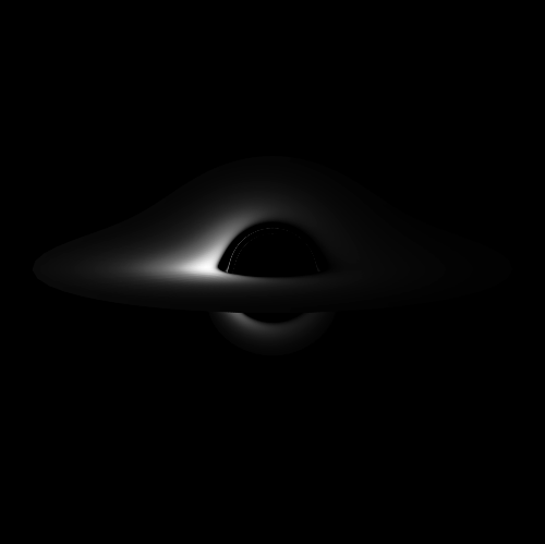
ax = bh.plot() # Create image like above
To sample photons on the accretion disk:
bh.sample_photons(100)
bh.photons
radius  alpha   impact_parameter    z_factor    flux_o
10.2146 5.1946  1.8935              1.1290      1.8596e-05
... (99 more)
Note that sampling is biased towards the center of the black hole, since this is where most of the luminosity comes from.
📝 Background
Swarzschild black holes have an innermost stable orbit of $6M$, and a photon sphere at $3M$. This means that the accretion disk orbiting the black hole emits photons at radii $r>6M$. As long as the photon perigee in curved space remains larger than $3M$ (also called the photon sphere), the photon is not captured by the black hole and can in theory be seen from some observer frame $(b, \alpha)$. The spacetime curvature is most easily interpreted as a lensing effect between the black hole frame $(r, \alpha)$ and the observer frame $(b, \alpha)$. The former are 2D polar coordinates that span the accretion disk area, and the latter are 2D polar coordinates that span the "photographic plate" of the observer frame. Think of the latter as a literal CCD camera. The photon orbit perigee and the radius in observer frame $b$ are directly related:
$$b^2 = \frac{P^3}{P-2M}$$
This makes many equations significantly more straightforward.
The relationship between the angles of both coordinate systems is trivial, but the relationship between the radii in the two reference frames is given by the monstruous Equation 13:
$$\frac{1}{r} = - \frac{Q - P + 2M}{4MP} + \frac{Q-P+6M}{4MP}{sn}^2\left( \frac{\gamma}{2}\sqrt{\frac{Q}{P}} + F(\zeta_\infty, k) \right)$$
Here, $F$ is an incomplete Jacobian elliptic integral of the first kind, $k$ and $Q$ are a function of the perigee $P$, $\zeta$ are trigonometric functions of $P$, and $\gamma$ satisfies:
$$\cos(\gamma) = \frac{\cos(\alpha)}{\sqrt{\cos^2\alpha + \cot^2\theta_0}}$$
In curved spacetime, there are usually multiple photon orbits that originate from the same coordinate and project to the ibserver frame (see e.g. gravitational lensing and Einstein crosses). Photon orbits that curve around the black hole and reach the observer frame are called "higher order" images, or "ghost" images. In this case, $\gamma$ satisfies:
$$2n\pi - \gamma = 2\sqrt{\frac{Q}{P}} \left( 2K(k) - F(\zeta_\infty, k) - F(\zeta_r, k) \right)$$
These ghost photons are what you see on the lower half of the image above, as well as the barely visible halo of light that wraps thinly around the photon sphere. For inclinations that are less edge-on, this ghost image is less pronounced though.
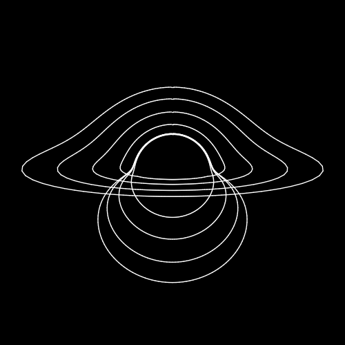
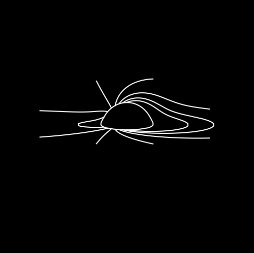
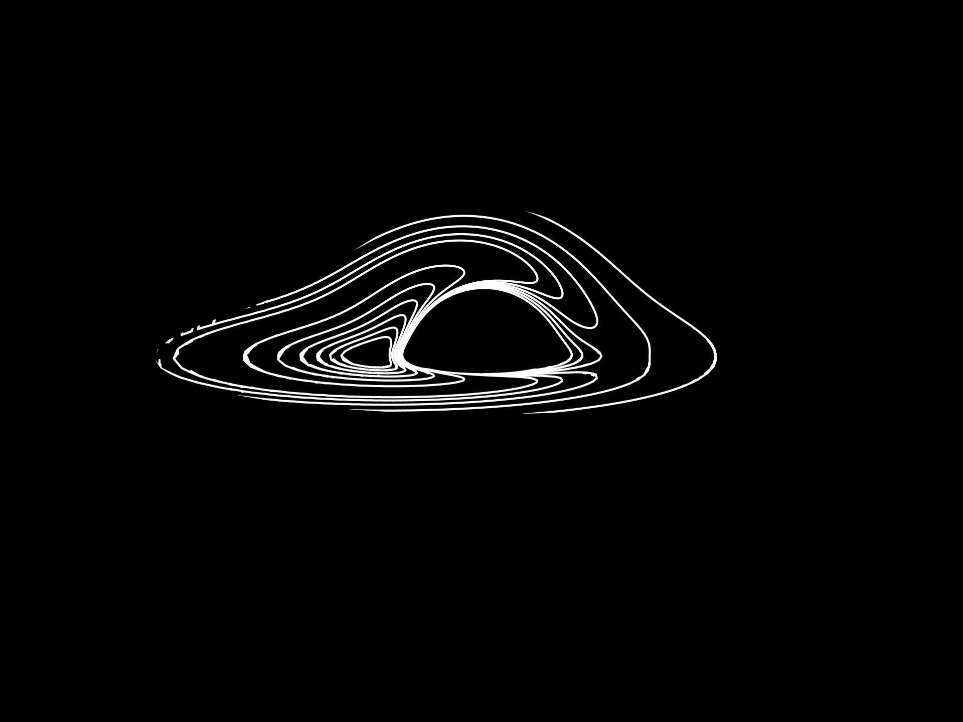
This repo uses scipy.optimize.brentq to solve these equations, and provides convenient API to the concepts presented in Luminet (1979). The BlackHole class is the most obvious one, but it's also educative to play around with e.g. the Isoradial class: lines in observer frame describing photons emitted from the same radius in the black hole frame. The Isoredshift class provides lines of equal redshift in the observer frame.
📕 Bibliography
[1] Luminet, J.-P., “Image of a spherical black hole with thin accretion disk.”, Astronomy and Astrophysics, vol. 75, pp. 228–235, 1979.
[2] J.-P. Luminet, “An Illustrated History of Black Hole Imaging : Personal Recollections (1972-2002).” arXiv, 2019. doi: 10.48550/ARXIV.1902.11196.
[3] Don N Page and Kip S Thorne. Disk-accretion onto a black hole. time-averaged structure of accretion disk. Astrophys. J., 191:499, July 1974.
1 maintainer

Metadata
1 maintainer
Release files for luminet 0.2.3
For a detailed explanation of source distributions (sdists) and built distributions (wheels), please see the package formats documentation.
Source distribution (sdist)
| File | Size | Uploaded | |
|---|---|---|---|
| luminet-0.2.3.tar.gz | 1.3 MB | Details |
Built distribution (wheel)
| File | Interpreter | ABI | Platform | Reset |
|---|---|---|---|---|
| luminet-0.2.3-py3-none-any.whl | Python 3 | none | any | Details |
Total release size: 1.4 MB
Release files / luminet-0.2.3.tar.gz
| Download URL | luminet-0.2.3.tar.gz |
|---|---|
| Size | 1.3 MB |
| Tags | Source |
|
SHA-256 checksum How to use checksums |
42fa9b8e18b20f3e92c66532cb8f234dcc6ce70de208193b13fd1d71a362dfe0
|
|
BLAKE2b-256 checksum How to use checksums |
88815f655439634e19b02779f43fa57cf559485335acc6f11fb30807e74532e1
|
| Upload date | |
|
Uploaded using Trusted Publishing? What is trusted publishing? |
Yes |
| Uploaded via |
twine/6.1.0 CPython/3.13.7
|
Provenance
Provenance describes where a file came from. On PyPI, provenance is shared via attestations, which provide a verifiable record of the build or publishing details. View details, limitations and caveats.


PyPI Publish Attestation
PyPI verified that this artifact, at this checksum, originated from the publisher listed below.
Signed by GitHub Actions, verified by PyPI on Jan 13, 2026.
Transparency logRelease files / luminet-0.2.3-py3-none-any.whl
| Download URL | luminet-0.2.3-py3-none-any.whl |
|---|---|
| Size | 25.8 kB |
| Tags | Python 3 |
|
SHA-256 checksum How to use checksums |
bf2a0d0ba79456efb70a7b1d2dc3ed6d9ac357b5b35b4d1c93bd9a482fd1261a
|
|
BLAKE2b-256 checksum How to use checksums |
921ed3586d64417cdcd243e9d73244fc8229ecf69f15f31ad7969965f30194be
|
| Upload date | |
|
Uploaded using Trusted Publishing? What is trusted publishing? |
Yes |
| Uploaded via |
twine/6.1.0 CPython/3.13.7
|
Provenance
Provenance describes where a file came from. On PyPI, provenance is shared via attestations, which provide a verifiable record of the build or publishing details. View details, limitations and caveats.
PyPI Publish Attestation
PyPI verified that this artifact, at this checksum, originated from the publisher listed below.
Signed by GitHub Actions, verified by PyPI on Jan 13, 2026.
Transparency log













