
Luxar







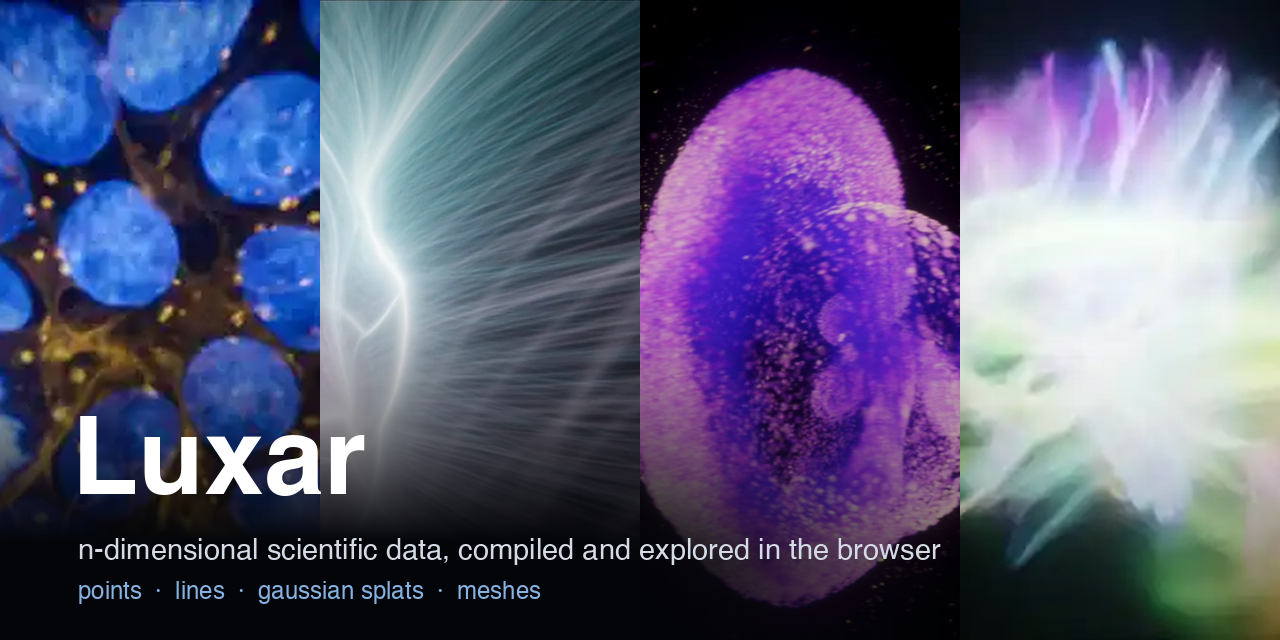
Compile n-dimensional scientific data once in Python. Explore gigabytes of it in any browser.
Luxar turns a scene you describe in Python (points, lines, triangle meshes, and image volumes fitted as Gaussian splats) into a chunked, spatially indexed Zarr archive that any static file host can serve and any WebGL2 browser can stream. Time, channel, or any other axis is a real dimension of the scene, not a folder of frames. It is built for microscopists with gigabyte volumes and time-lapses, and for anyone with more points, tracks, or dimensions than a desktop viewer will hold.

A Drosophila embryo through gastrulation: 500 light-sheet timepoints, 256K Gaussian splats each, streamed from static hosting and played in the browser. Open it live. Recording by the Keller lab, HHMI Janelia.
Three ideas carry most of the design:
- Compile, don't load. Ordering, chunking, compression, and levels of detail happen once, at compile time. The viewer fetches only the chunks the current view touches and starts drawing while the rest arrives.
- n dimensions are first class. Time, channel, camera, or an abstract axis is a dimension with units and extent. Hidden axes become sliders and toggles, and geometry is sliced by nD proximity.
- Represent, don't rasterize. An image volume is fitted with sparse oriented Gaussians and shipped as geometry rather than voxels: a 3.6 GB light-sheet stack becomes 2 MB, a 400-timepoint time-lapse 81 MB.
demos.luxarviewer.dev hosts 88 live demos
with nothing to install. Already have a scene? Open it in the hosted viewer at
https://luxarviewer.dev/?src=<url>. To build your own, start at
Quick start; if your data is an image volume, start at
Volume rendering.
How it works · Quick start · Your first scene · Gallery · Volume rendering · Geometry · Scene graph · nD data · Sharing · Viewer · Format and architecture · Develop · Docs · Cite
How it works
Everything expensive happens before anyone opens a browser. The compiler orders each node along a space-filling curve (a mesh has none: it loads whole), cuts it into chunks of about 64 KB, compresses them, writes an nD spatial index and levels of detail, and, for image volumes, runs the Gaussian fit. The viewer's job is reduced to fetching the chunks a view needs and drawing them, so what remains at exploration time is bounded by your graphics card, your screen, and your network link rather than by the size or format of the file.
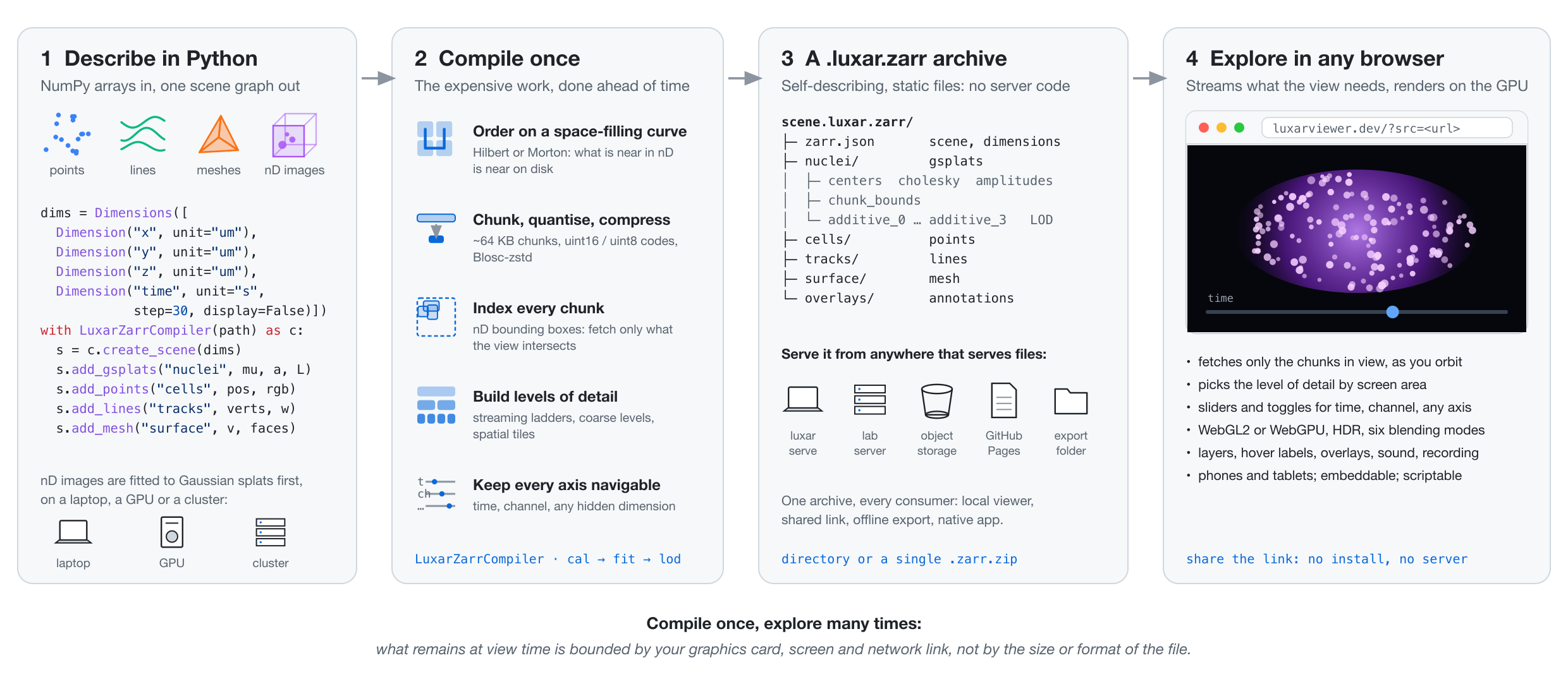
The four stages, left to right: describe the scene in Python, compile it once, host the archive as static files, explore it in any browser.
| Capability | What you get |
|---|---|
| Four geometries | Points, lines, Gaussian splats, and triangle meshes share one attribute model: nD positions, colors, and opacity, plus a per-element size for all but meshes |
| n dimensions | Named axes with physical units, radius-based slicing, keyboard navigation, per-axis transforms |
| Scale | Interactive frame rates up to about 10 million primitives, with levels of detail and progressive streaming from local files or remote hosts |
| Volume rendering | Image volumes fitted to oriented Gaussians: gigabytes of voxels become megabytes of streamable, GPU-native geometry, time-lapses included |
| Appearance | HDR 16-bit float color, bloom and tone mapping, matplotlib and colorcet colormaps, six blending modes from additive to physically based emission and absorption |
| Fitting pipeline | cal → fit → lod with cross-validated splat budgets, optional CUDA or Apple MPS, whole-time-lapse fitting across many GPUs or a Slurm cluster |
| Interoperable | Reads classical 3D-Gaussian-splatting captures (INRIA, .splat, .spz, SuperSplat, PlayCanvas SOG); writes INRIA PLY |
| Shareable | Any static host serves a scene; luxar export writes an offline folder or a native macOS or Linux app that opens with no install |
| Requirement | Notes |
|---|---|
| Python | 3.12 or newer |
| Operating system | macOS and Linux are developed and tested on; Windows is untested |
| Browser | WebGL2 (Chromium, Firefox, and WebKit engines are smoke-tested; see Using the viewer) |
| GPU | Not needed to view. Optional for fitting splats: NVIDIA CUDA or Apple MPS make it much faster than the CPU path |
| Node.js 22 | Only to develop the viewer; users never need it |
Scope. Luxar does not ray-march voxels: volumes are fitted, and the fit is lossy in a measured way. It is a visualization system, not an annotation or segmentation tool, and it needs a browser with WebGL2. Fitting a large time-lapse wants a GPU; viewing one does not.
Status. Luxar is versioned by calendar date and released from main;
what stays stable across releases and how breaking changes are announced is in
the compatibility policy, and every
change is in the changelog.
Quick start
pip install luxar       # viewer, compiler and CLI; add "luxar[gsplats]" to fit volumes
luxar demo              # Browse the 90 bundled demos
luxar demo run cloud    # Run one: generates the data and opens the viewer
Some demos need extra packages; luxar demo deps --install fetches what a demo
reports missing. To work on Luxar itself, or to run from a source checkout:
git clone https://github.com/royerlab/luxar.git
cd luxar
make setup-dev          # Auto-installs Node.js, pnpm, Hatch (no sudo)
hatch shell             # Activate the environment setup-dev created; then the same commands
luxar demo run cloud builds a convective cloud, a 4D point cloud that evolves
over a time axis, and opens it in the viewer, where the time slider plays it
back:

The whole thing in one take: pip install luxar, then luxar demo run cloud.
Where to go next depends on your data. An image volume or a time-lapse of
volumes: Volume rendering. Points,
tracks, or embeddings: Your first scene. A mesh file:
luxar mesh import under Geometry types. A 3D-Gaussian-splatting
capture: luxar gsplat import under Volume rendering.
The demo catalog and the luxar demo commands
luxar demo prints every bundled demo, grouped by category: index, key,
geometry, what it needs, and whether you have already built it.
🎬 90 Luxar demos  ·  75 built  ·  8 cached  ·  7 not generated yet

 ASTRONOMY ──────────────────────────────────────────────────────────── 6 demos
 ✓  2  asteroids_solar_system                  points+lines  300 MB
 ✓ 12  cosmicflows_laniakea                    points+lines  25 MB
 • 15  desi_galaxies                           points        73 MB
 ...

 MEDICAL ────────────────────────────────────────────────────────────── 4 demos
 ✓ 17  dmri_tractography                       lines         588 MB
 • 29  gsplats_2d_cmu1_pathology               gsplats       150 MB GPU?
 ...

 SYNTHETIC ─────────────────────────────────────────────────────────── 18 demos
 ✓ 10  cloud                                   points
   11  collision                               points
 ...
 ✓ 22  exotic_surfaces                         points

 ✓ built   • inputs cached   (blank) not generated yet
 GPU/GPU? = required/optional     git-lfs kaggle manual = data you supply

 Run      luxar demo run <key|#>                e.g. luxar demo run cloud
 Details  luxar demo info <key|#>
 Filter   luxar demo list -c astronomy -g gsplats
 Deps     luxar demo deps                       --install fixes what it reports
 Caches   luxar demo cache list                 cache clear <key> to reclaim
 Stop     luxar demo stop                       frees ports of forgotten runs
The left rail is what you already have: ✓ the scene is built, • the
inputs are downloaded, blank means neither, so a second pass over the catalog
shows exactly what is on disk. The last column is what a demo costs you
before you commit to it: the download size, GPU (required) or GPU?
(optional), plus git-lfs, kaggle, or manual when it needs Git-LFS data,
Kaggle credentials, or a file you supply.
The luxar demo commands
| Command | What it does |
|---|---|
luxar demo |
Browse the catalog (same as luxar demo list) |
luxar demo list -c microscopy |
Filter by category: synthetic, microscopy, embeddings, photogrammetry, astronomy, structural, networks, medical, geoscience, genomics, connectome |
luxar demo list -g gsplats |
Filter by geometry: points, gsplats, lines, mesh, points+lines, mixed |
luxar demo info <key|#> |
Requirements, caches, outputs, and how to run one demo |
luxar demo run <key|#> |
Run by key (e.g. luxar demo run lorenz) or by the index shown in the table — keys are stable, indices shift as demos are added |
luxar demo run <key> -- ARGS |
Forward arguments to the demo script, e.g. luxar demo run gsplats_3d_tribolium_embryo -- --recompute --no-serve |
luxar demo run-all |
Build every eligible demo's dataset unattended. Manual/Kaggle-data demos are always skipped; GPU-required demos, downloads over 200 MB, and already-built outputs are skipped by default (--include-gpu, --max-download-mb 0, --force lift these) |
luxar demo cache list |
Inventory the demo caches under ~/.cache/luxar/, with sizes and orphans |
luxar demo cache clear <keys> |
Reclaim space — --all for everything, --outputs to drop generated scenes too, --dry-run to preview |
Demos run as subprocesses, so Ctrl-C tears down the demo and the viewer it
spawned. Every tile in the Gallery is one of these demos; pick a key
from luxar demo and luxar demo run <key> reproduces it locally.
Your first scene
Define a coordinate system, add geometry, and the compiler writes a
.luxar.zarr archive:
import numpy as np
from luxar import LuxarZarrCompiler, Dimensions, Dimension

# Define coordinate system
dims = Dimensions([
    Dimension("x", unit="um", display=True),
    Dimension("y", unit="um", display=True),
    Dimension("z", unit="um", display=True),
])

# Create and save visualization
with LuxarZarrCompiler("my_data.luxar.zarr") as compiler:
    scene = compiler.create_scene(dimensions=dims)

    # Your data as NumPy arrays
    positions = np.random.randn(100_000, 3).astype(np.float32) * 50
    colors = np.random.rand(100_000, 3).astype(np.float32)

    scene.add_points("MyPoints", positions, colors=colors)
luxar serve my_data.luxar.zarr --viewer --open   # data server + viewer, opens the browser
luxar info my_data.luxar.zarr --stats            # what you compiled, including the chunk layout
luxar serve my_data.luxar.zarr --profile 3g --viewer   # how it behaves on a slow link
luxar export my_data.luxar.zarr -o my_export/    # a folder a colleague opens without installing Luxar
(From a source checkout, luxar export needs make build-viewer once.) To publish the scene as a link, see
Sharing and hosting a scene.
Gallery











A cross-section of the bundled demos, all four geometry types across real scientific datasets. Each tile is an orbit preview: click the image for the video, or the title to open that scene live at demos.luxarviewer.dev. Each data tile carries a short credit; full citations and licenses are in ACKNOWLEDGMENTS.md. Tiles with no credit are synthetic.
Gaussian splats: microscopy, medical, and astronomy
 |
 |
 |
|---|---|---|

| Cells3D multichannel fluorescence Allen Institute for Cell Science |
Mouse Blastocyst Lamin B1 + DAPI Blin et al. 2019 |
Zebrafish Neuromast 4D timelapse Jacobo lab, CZ Biohub |
 |
 |
 |
| Tribolium Embryo light-sheet Barry et al. 2022 |
CT Anatomy Atlas TotalSegmentator Wasserthal et al. 2023 |
Milky Way Dust galactic dust clouds Leike et al. 2020 |
The living cell & genome
 |
 |
 |
|---|---|---|
| FlyWire Connectome fly-brain neurons Dorkenwald et al. 2024 |
Single-Cell 3D Genome Dip-C chromosomes Tan et al. 2018 |
C. elegans 4D nuclei-tracking timelapse Santella et al. 2022 |
 |
 |
 |
| ATP Synthase molecular machine Zhou et al. 2015 |
Tabula Sapiens human cell atlas Tabula Sapiens Consortium 2022 |
Human Multiome ATAC-peak UMAP Domcke et al. 2020 |
 |
 |
|
| White-Matter Tractography 87 human dMRI tracts Yeh 2022 |
Cells3D Isosurfaces shaded membrane + nuclei surfaces Allen Institute for Cell Science |
Earth & geoscience
 |
 |
|---|---|
| Global Earthquakes USGS on the globe USGS catalog; NASA Blue Marble |
Rivers of Earth topography + river networks HydroSHEDS + NOAA NCEI |
Networks & embeddings
 |
 |
 |
|---|---|---|
| CAIDA Internet AS topology CAIDA, UC San Diego |
HuRI human interactome Luck et al. 2020 |
Protein Landscape CAFA5 embeddings CAFA5; Elnaggar et al. 2022 |
 |
 |
|
| Spotify audio-feature embedding Spotify Web API |
Zebrahub multiome embedding Kim et al. 2024 |
Synthetic & mathematical
 |
 |
 |
|---|---|---|
| Lorenz Attractor chaotic dynamics |

Rainbow Sphere HDR Fibonacci sphere |

Quantum Orbitals hydrogen 2p_z |
 |
 |
 |



| Spiral Galaxy barred multi-armed disk |
Galaxy Simulation density-wave spiral |

Hilbert Curve 3D space-filling |
 |
 |
|

| Particle Collision physics event |

Ocean bioluminescent jellyfish |
The curated set lives in scripts/gallery/manifest.json and make generate-gallery
regenerates the media. A few heavy scenes (the DESI cosmic web, the Gaia
catalog) have no tile here because they need a GPU to capture or data you must
fetch yourself; every tile is a bundled demo, so luxar demo run <key>
reproduces it and luxar demo run-all builds every eligible one (it always
skips manual/Kaggle data, and by default skips GPU-required demos, downloads over
200 MB, and already-built outputs).
Volume rendering with Gaussian splats
An image volume is a grid of voxels; a modern light-sheet timepoint is several gigabytes of them, and a time-lapse is hundreds of timepoints. Luxar does not ship that grid. It fits the volume with a sparse mixture of oriented 3D Gaussians and renders those instead, so the size of the representation follows how much structure the sample contains rather than the grid it was sampled on. Empty space costs nothing, and what is left is small enough to stream:
| Dataset | Source volume | Fitted representation |
|---|---|---|
| Tribolium embryo — light-sheet, 1 timepoint | 965 × 1871 × 991 = 1.8 G voxels (3.6 GB as TIFF) | 296,559 splats · 2.0 MB |
| C. elegans embryo — confocal, 400 timepoints | 400 × 41 × 512 × 512 = 4.3 G voxels | 5.64M splats · 81 MB (about 200 KB per timepoint) |
The C. elegans fit is fetched from the permissively licensed Zenodo demo record (see Where the demo data lives); the Tribolium fit is produced locally because its source is not redistributable. Both use full source resolution, and the single-file Tribolium fit works out to about 7 bytes per splat on disk. Both render in any WebGL2 browser: no 3D textures, no ray-marching, and no CUDA on the viewing machine.

A raw Drosophila light-sheet stack in napari, luxar gsplat fit converging (training PSNR plotted as it runs), a dozen lines of Python to compile the scene, and the result opening in the browser. Excerpts of Supplementary Video 1.
The pipeline: cal, fit, lod
# 1. Choose the splat budget K* by blind-spot cross-validation
luxar gsplat cal volume.tiff cal.json

# 2. Fit at K*
luxar gsplat fit volume.tiff fit.gsplats.zarr --seeds <K*>

# 3. Build the streaming topology
luxar gsplat lod fit.gsplats.zarr scene.gsplats.zarr --recipe stream
cal sweeps the splat count, finds where held-out PSNR peaks, and reports the
dataset's noise floor, so the budget is chosen by cross-validation against the
data rather than by guesswork. Inputs can be .zarr, .zarr.zip, OME-Zarr,
.tiff, .npy, or .npz, with --timepoint, --channel, and --array-key to
pick a slice of a larger store. luxar gsplat compare reports PSNR, SSIM, and
MSE of a fit against its source.
Fitting hardware. Fitting needs the gsplats extra (pip install "luxar[gsplats]", or pip install -e ".[gsplats]" from a checkout). It runs on the CPU, and much faster on an NVIDIA
GPU (make build-cuda compiles the CUDA kernels for your card; they cannot ship in
the wheel) or on Apple silicon through MPS. Seeding and the optional non-local-means
denoising follow the same device choice. On a cluster, make build-cuda SLURM=1
builds the extension on a GPU node; if a fit logs "GPU fitting will use slower
PyTorch fallback", it still runs, just without the compiled kernels. Viewing never
needs any of this.
Every option, with examples, is in the CLI package README; the fitting model and the LOD algorithms are in the Gaussian splatting README.
Scaling: pick a topology, stream the rest
luxar gsplat lod --recipe turns a fitted dataset into a level-of-detail
topology. The recipes are named by intent and ordered by dataset scale:
| Recipe | Structure | Use when |
|---|---|---|
flat |
one bare leaf | tiny data, debugging |
stream |
one leaf + progressive ladder | small data, fast first paint |
levels |
coarse→fine replacement levels | zooming across scales |
tiles |
spatial tiles, each with its own ladder | large scene at one scale |
overview |
instant coarse overview, fine tiles on zoom | huge scene, "see everything first" |
adaptive |
tiles where every tile picks its own level | largest scenes, locally adaptive |

One Tribolium fit, six topologies side by side (flat, stream, levels, tiles, overview, adaptive), every column but flat colored by the part or level it is drawn from; the data-loading monitor counts what is resident as the camera dollies in. Open the demo or watch Supplementary Video 7.
Apart from flat, every recipe carries a progressive streaming ladder by
default: splats are reordered so that early prefixes carry as much of the signal
as possible, so the first chunk to arrive is already a meaningful picture and
later chunks refine it. Where levels replace each other, the viewer picks between
them by the screen area the object occupies, a viewport fraction that needs no
per-resolution tuning: the finest level shows while the object fills at least
half the screen, each halving of occupied area steps one level coarser, and the
partition-bound recipes (adaptive, overview) anchor one step higher.
Time-lapses are one dataset, not a folder of frames
Each timepoint is fitted in 3D and the results are stacked onto a time axis:
every splat gains a time coordinate and a matching covariance entry (zero width
for a discrete axis, a real extent if you want temporal spread), so a complete 4D
acquisition (or 5D, adding channel or camera) lives in a single .gsplats.zarr.
The viewer's time slider is ordinary nD slice navigation, and because splats are
stored timepoint-major, each frame's splats are contiguous on disk: scrubbing
fetches the chunks of the current frame and nothing else (at most the one chunk
on a frame boundary carries a few splats of its neighbor). Coarsening treats the
time and channel axes as hard barriers: coarse splats are never merged across
them and mass is conserved per barrier group, so a timepoint keeps its exact
brightness at every level of detail and scrubbing never smears one frame into
the next.
Fitting a whole time-lapse is one command, on whatever hardware you have:
# Every GPU in the box, planned over T×C, resumable
luxar gsplat batch-fit run movie.zarr out/ --gpus auto

# Or a Slurm array job on a cluster
luxar gsplat batch-fit submit movie.zarr out/ -p gpu --tiling content --cal cal.json
Both plan tiles once across all timepoints and channels, fit each tile as an
independent task, then stream-merge the results, so peak memory is one tile
region, never the whole movie. status, validate, merge, and cancel are
shared by both backends; --merge-recipe gives each spatial part its own LOD
ladder as it streams.
Emission and absorption, not just glow
The volumetric blending mode implements the emission-absorption model of direct
volume rendering (Max 1995) in closed form for Gaussians. One per-layer knob,
absorption κ, morphs the render continuously:
| κ | Look | Good for |
|---|---|---|
0 |
pure emission, bit-identical to additive |
sparse fluorescence, X-ray-like projection |
| small | attenuated projection: near structure pops, occluded structure dims | depth cueing in dense time-lapses |
| large | dense smoke- or ink-like medium | opaque tissue, anatomy |
Because fitted amplitudes are background-relative image intensities rather than learned opacities, κ reads as an effective turbidity of the sample instead of an arbitrary rendering constant, and absorption is orientation-consistent: an elongated splat seen end-on absorbs more than the same splat seen side-on. Points, lines, and Gaussian splats all render the same physics, on both the WebGL and the WebGPU backend.
luxar gsplat convert fit.gsplats.zarr scene.luxar.zarr \
    --blending-mode volumetric --absorption 4 --colormap plasma --tone-mapping ACES
The other modes cover the classical spectrum: additive and luminous (pure
emission; additive is the default), max (maximum-intensity projection), and
normal and opaque (surfaces). The derivation is in the
Volumetric Blending Spec.
Photogrammetric splats, too
The same renderer reads classical 3D-Gaussian-splatting captures. luxar gsplat import auto-detects INRIA .ply, antimatter15 .splat, Niantic and Scaniverse
.spz, SuperSplat compressed .ply, and PlayCanvas SOG, then feeds them through
the same LOD and streaming path; the largest interop demo is a 13.6M-Gaussian
aerial city. luxar gsplat export writes INRIA PLY back out.
How faithful is it
The fit is lossy, so fidelity is measured rather than asserted. Across a
17-volume microscopy benchmark (4 to 107 million voxels; spinning-disk, confocal,
light-sheet, and iSIM), fits at each volume's cross-validated splat budget land
between 26 and 67 dB PSNR at 6 to 340 times compression (median 99), where
compression is the source volume at its stored bit depth over the stored splat
archive. The benchmark, the cross-validation protocol, and the residual analysis
are in the preprint (see Citation); luxar gsplat compare reports the
same metrics for your own data. The Tribolium fit above is a gigavoxel source
outside the benchmark's per-volume range, so its ratio exceeds that ceiling; the
C. elegans figure aggregates 400 timepoints of 10.7 M voxels each.
Geometry types
Points
Collections of nD points rendered as soft-edged spheres.
scene.add_points(
    "ParticleCloud",
    positions,           # (N, D) float32 - nD coordinates
    colors=colors,       # (N, 3) float32 - RGB (0-1, HDR supported)
    radii=radii,         # (N,) float32 - per-point size
    sharpness=sharpness, # (N,) float32 - edge falloff (0-1, normalized)
    opacity=0.8,         # Global opacity
    # "additive" (default), "volumetric", "normal", "max", "opaque", "luminous"
    blending_mode="additive",
)
Lines
Connected segments with per-vertex attributes: tracks, trajectories, skeletons.
scene.add_lines(
    "Branches",
    vertices,      # (N, D) float32 - nD vertex positions
    widths=widths, # (N,) float32 - per-vertex width
    colors=colors, # (N, 3) float32 - per-vertex colors
)
Gaussian splats
Oriented Gaussian functions, Luxar's volume-rendering primitive. Fit them with
the pipeline above and add the result with scene.add_gsplats_from_data(name, result) or scene.add_gsplats_from_file(name, "fit.gsplats.zarr"); embedding an
existing fit needs no extra dependency.
Mesh
Triangle surfaces: isosurfaces, segmentation boundaries, cortical and organ meshes. The other three primitives are soft and emissive; a mesh is the one connected, shaded type, lit by a view-anchored key so shape reads from shading rather than density.
scene.add_mesh(
    "Nuclei",
    vertices,               # (V, D) float32 - nD vertex positions
    faces,                  # (F, 3) uint32  - triangle vertex indices
    normals=normals,        # (V, 3) float32 - optional, needs normal_dims
    normal_dims=[0, 1, 2],  # which three dims the normals describe
    colors=colors,          # (V, 3|4) - optional per-vertex RGB(A)
)
A mesh has no per-element size (its extent comes from its vertices) and renders
with opaque blending by default, which makes it depth-correct without sorting.
Normals are optional: omit them and the shader derives flat per-face normals;
pass them and normal_dims says which three dimensions they describe. Already
have a mesh file? luxar mesh import reads PLY, OBJ, STL, VTP, and glTF/GLB with
no extra dependencies, and a directory of T<number>-indexed files stacks into a
mesh time-lapse:
luxar mesh import bunny.ply bunny.luxar.zarr
luxar mesh import frames/ frames.luxar.zarr --pattern '*.ply'
luxar mesh lod bunny.luxar.zarr bunny_lod.luxar.zarr -L 4   # coarse levels
luxar serve bunny_lod.luxar.zarr --viewer
Meshes support spatial partitioning (partition=), decimated coarse levels
(substitutive_lod=, built by luxar.mesh.decimate), and a spatially coherent
reveal ladder (additive_lod={"method": "radial"}), though only one of the three
per mesh; an additive ladder over an arbitrary order and volumetric blending
are refused with an explanation rather than degraded silently (a volumetric
inherited from a parent falls back to opaque with a warning). The reasons are
in the mesh spec.
Scene graph and transforms
Nodes live in groups, groups nest, and transforms compose down the tree. A 4×4
transform moves geometry through the three displayed dimensions:
from luxar import transforms

# Basic transforms
t = transforms.translate(10, 0, 0)
r = transforms.rotate_z(45)
s = transforms.scale(2, 2, 2)

# Compose (applied left-to-right)
combined = transforms.compose(t, r, s)

# Apply to groups
group = scene.add_group("Cluster", transform=combined)
scene.add_points("Points", positions, parent=group)

# Hierarchical transforms
parent = scene.add_group("Robot")
parent.transform = transforms.translate(100, 0, 0)

arm = parent.add_group("Arm")
arm.transform = transforms.rotate_y(45)  # Relative to parent
The separate nd_transform does the same for the non-displayed dimensions, so
two datasets recorded on different clocks, sampling rates, or channel orders can
be aligned in one scene instead of being resampled first. Continuous and discrete
axes take an affine scale and offset; categorical axes take a permutation:
group = scene.add_group(
    "DatasetB",
    transform=transforms.translate(10, 0, 0),      # displayed dims (4x4)
    nd_transform={
        "time": {"scale": 0.001, "offset": 50.0},  # ms → s, shifted
        "channel": {"permutation": [2, 1, 0]},     # reorder channels
    },
)
group.add_points("cells", positions_5d)            # children inherit it
The viewer applies these by inverse-transforming the query (slice position and tolerance) from world to local space once per view change rather than transforming millions of coordinates; see the nD Transforms Spec.
n-dimensional data
Every axis of a scene is declared once, with a unit, an extent, and whether it is displayed or navigated:
dims = Dimensions([
    # Displayed dimensions (shown in 3D viewer)
    Dimension("x", unit="um", range=(-100, 100), display=True),
    Dimension("y", unit="um", range=(-100, 100), display=True),
    Dimension("z", unit="um", range=(-50, 50), display=True),

    # Non-displayed dimensions (navigated via sliders)
    Dimension("time", unit="s", range=(0, 60), step=1.0, display=False),
    Dimension("channel", unit="", categories=["DAPI", "GFP", "mCherry"], display=False),
])
Points in nD are treated as hyperspheres: an element is visible in the current
3D slice when its hypersphere intersects it, and for axes declared spatial=True
(hidden axes default to non-spatial) its effective radius shrinks with distance
d from the slice as sqrt(r² - d²). Every non-displayed
axis becomes a control in the viewer: a slider for continuous and discrete axes,
a toggle or dropdown for categorical ones. Press 1 to 9 to select a hidden
axis, [ and ] to step it, and N to open the dimension panel.

The Dimension Navigation panel driving the time axis of the C. elegans nuclei-tracking scene (splats for nuclei, lines for tracks): time is a hidden dimension, played like any other. Excerpt of Supplementary Video 12.
Sharing and hosting a scene
A compiled scene is a folder of static files, or a single .luxar.zarr.zip.
Any host that serves files over HTTPS can publish it, with no server code to
run: upload the store and share https://luxarviewer.dev/?src=<URL of the store>.
The host needs two things:
- CORS. The viewer page comes from
luxarviewer.devwhile the data comes from your host, so the host must sendAccess-Control-Allow-Origin(*is fine for public data). Without it the scene stays empty and the browser console shows requests blocked by CORS policy, not a 404. - Byte ranges, for zipped stores only. A
.luxar.zarr.zipis read in place withRangerequests, so the host must honor them, allow theRangerequest header, and exposeContent-Range,Content-Length,Accept-Ranges, andETag. A directory store uses plain GETs and needs only CORS.
Typical options, roughly from most to least convenient for scenes of a few GB:
- Cloudflare R2 (what serves the demo corpus at
data.luxarviewer.dev): object storage with no egress fees, a free tier of about 10 GB, public buckets, custom domains, and a CORS policy pasted in the dashboard. Reads are billed per request, so chunk size matters (see below). Watch out: a custom domain needs a Cloudflare-managed DNS zone. Check the free tier before publishing terabytes. - Amazon S3 / Google Cloud Storage: same static-object model; the S3 CORS JSON in the Viewer Guide applies to S3 and R2 as is, and GCS takes the equivalent through
gsutil cors set. Watch out: egress is billed per GB, which is the cost that grows with popularity. - GitHub Pages: free, versioned, zero setup for small scenes (commit the store to a
gh-pagesbranch). CORS and byte ranges work out of the box. Watch out: files above 100 MB are rejected and Git LFS objects are not served, so it suits scenes under a few hundred MB in total. Drop a.nojekyllfile at the site root, or Jekyll strips the dotfiles a zarr-v2 store and.luxar-index.jsondepend on. - Your lab's web server (nginx, Apache): data stays on infrastructure you control; an nginx snippet is in the Viewer Guide. Watch out: you add the CORS and range headers yourself; institutional proxies sometimes strip
Range. - No host at all:
luxar export scene.luxar.zarr -o out/writes the viewer plus a stdlib-onlyserve.py; from a source checkout, aftermake build-launchers,--native macosgives a double-clickable app (Distributing scenes). Watch out: the recipient runs it locally; nothing is shareable as a link.
An archive of record such as Zenodo is the right place to deposit a scene for citation; whether it can also serve it to the viewer depends on its CORS and range headers, so test before linking to it.
Object stores bill per request, and most generated stores land far below the
64 KB chunk target (the demo corpus averages 5 KB per file), so run
luxar optimize before
publishing and pick the profile by access pattern: local when the viewer will slice into a large node,
hosting or archive when it loads the node whole (one demo went from 9,390
requests to 2,348 on a cold load). The re-chunked store carries a new content
hash, so publish it under a new URL prefix rather than over the old one. To
verify a host: curl -sI -H "Origin: https://luxarviewer.dev" <URL> should
return an access-control-allow-origin header, and for a zipped store a ranged
GET (curl -s -o /dev/null -D - -H "Range: bytes=0-0" <URL>) should answer 206
(a HEAD may legitimately answer 200). The full host-by-host setup, the
.luxar-index.json
that makes a folder of scenes browsable, and the export and native-bundle paths
are in Distributing scenes, the
Viewer Guide,
and the Demo Site Runbook, which
documents how the demo corpus itself is served.
Using the viewer
| Key or input | Action |
|---|---|
| Left drag, right drag | Rotate, pan (the macOS default; the reverse elsewhere; swap them in the Navigation panel) |
| Scroll, Shift + scroll, Ctrl/Cmd + scroll | Zoom, roll, field of view |
V, F, Space |
Cycle orbit / fly / ortho, recenter, fullscreen |
W A S D, Alt+W/S, arrows, Q/E, I |
Fly mode: move, up and down, look, roll, inertia |
1 to 9, [ ], N |
Select a hidden dimension, step it, dimension panel |
L, R, M, T, P, O, H |
Layers, rendering, monitor, recording, performance, dataset browser, help (Ctrl+L: debug console) |
| URL parameter | Effect |
|---|---|
?src=<url> |
Scene to open |
?theme=dark|light|frosted-glass|liquid-glass |
Interface theme |
?renderer=webgl|webgpu |
WebGL2 (default) or the WebGPU backend |
?debug |
Expose window.__luxarDebug |
?noCache, ?clearCache, ?noPrefetch |
Disable the cache tiers, clear the persistent cache, disable prefetch |
If a scene stays empty, check the browser console: a CORS error means the host is refusing the data (see Sharing and hosting); a 404 means the URL is wrong. The panels, the camera modes, and every shortcut are described in the Viewer Guide.
Browser Compatibility
Luxar needs WebGL2; WebGPU is opt-in with ?renderer=webgpu and falls back to
WebGL2 when no adapter is available. The build targets esnext with no
browserslist, so there is no version floor to quote, only what has been run.
The end-to-end smoke subset passes on Playwright's three bundled engines:
| Engine | Smoke subset | Notes |
|---|---|---|
| Chromium | pass | Persistent (OPFS) cache tier active |
| Firefox | pass | Persistent (OPFS) cache tier active |
| WebKit | pass | Runs without the persistent cache tier, so Safari and the native launcher keep chunks in memory only (the cache panel shows the opfs-unavailable badge) |
Playwright's WebKit is not Safari, so Safari and Edge themselves are untested, and real phones and tablets are supported but unmeasured; touch input (one- and two-finger orbit, pinch, twist, tap-to-pick, long-press menus) is exercised by an emulated mobile suite. The dated run and how to reproduce it are in the viewer README.
Data format, performance, and architecture
A scene is a Zarr store (format 3 by default; format 2 is read and can be
written with LUXAR_ZARR_FORMAT=2) whose nodes carry their arrays, a spatial
index, and optional LOD ladders:
scene.luxar.zarr/
├── zarr.json               # Scene attributes and consolidated metadata
└── node_name/
    ├── zarr.json           # Node attributes (type, transform, rendering)
    ├── positions/          # (N, D) coordinates (quantized on disk, decoded as float32)
    ├── colors/             # (N, 3) RGB values
    ├── radii/              # (N,) point sizes
    └── chunk_bounds/       # Spatial index for efficient queries
The store is specified in LUXAR_ZARR_FORMAT.md and the fitted-splat container in GSPLATS_ZARR_FORMAT.md.
Rendering cost. On an NVIDIA RTX 3070 at 1280×720, with adaptive DPR pinned to 1.0 and the primitives drawn at the reference size (4 px for points and splats, 1.5 px for lines) through the default HDR pipeline, one synchronized render-and-readback call takes (milliseconds; the 60 FPS budget is 16.7):
| Elements | Lines | Points | Gaussian splats |
|---|---|---|---|
| 100K | 1.21 | 1.23 | 1.72 |
| 1M | 3.31 | 4.98 | 8.64 |
| 10M | — | 18.8 | 19.4 |
At ten million elements the call runs 12 to 16% over budget, and at that element density lowering the render resolution does not help (the cost tracks elements per pixel, not pixels), which is what the projected-density guard below is for. Typical scenes are lighter than these synthetic sweeps: the fifteen demo scenes of the same sweep all hold 60 FPS, the heaviest, a 2.2M-splat time-lapse frame, in 5.6 ms. Very large overdraw-bound scenes such as a 29.6M-splat whole-slide image are thinned by the projected-density guard (on by default). Load time is dominated by transfer and decode, so it follows your link and cache state rather than the element count. The whole-slide and Apple M4 Max measurements, and the method, are in the viewer performance audit.
Architecture. Luxar is two code bases that never import each other. The
Python package authors, fits, and compiles; the TypeScript viewer streams and
renders; the archive is the only contract between them, so anything that writes
it feeds anything that reads it: the hosted viewer, an offline export, an
embedded @luxar/viewer, a native launcher.
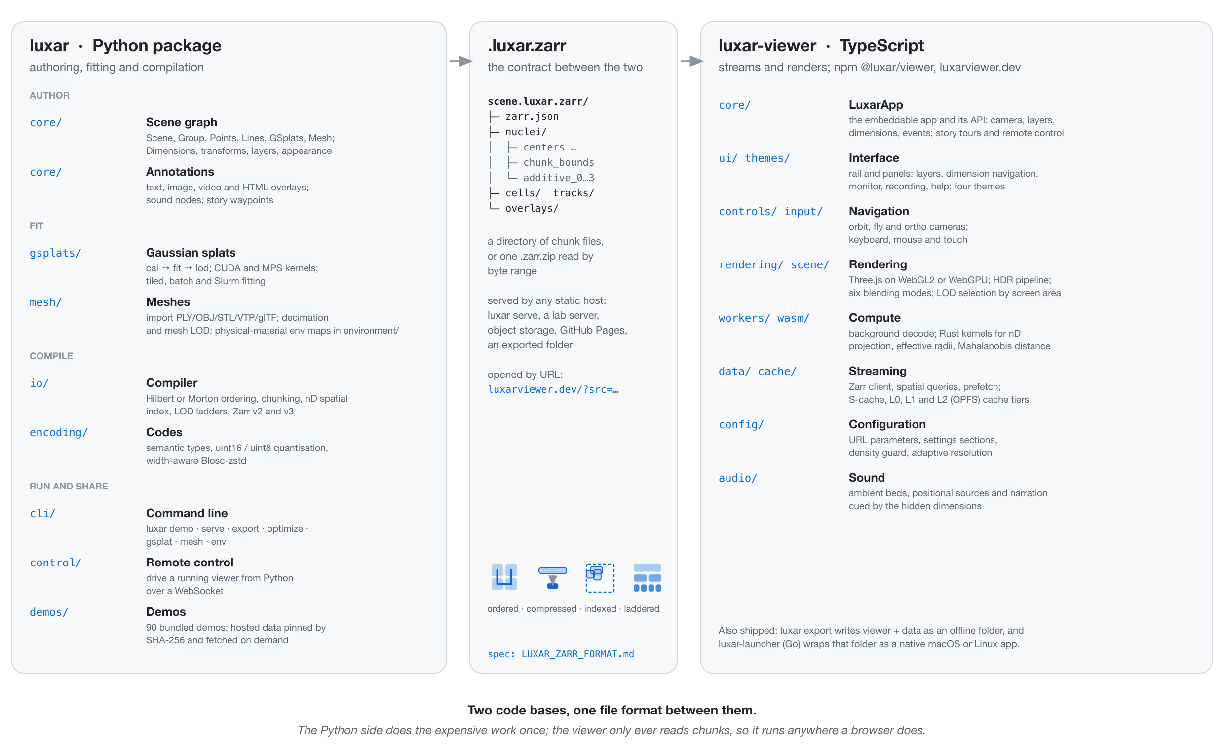
The Python package on the left, the viewer on the right, and the archive between them; each row names the module that owns it.
Python side. core/ is the scene graph a user builds: nodes for the four
geometry types, groups with transforms, Dimensions that declare every axis
with its unit and extent, per-node appearance, and annotations (text, image,
video and HTML overlays, sound, story waypoints). gsplats/ turns image volumes
into that geometry: cross-validated calibration, the fitter with its CUDA and
Apple-MPS kernels, tiled and multi-GPU batch fitting, and the LOD recipes.
mesh/ imports and decimates surfaces. io/ is the compiler: it orders every
node along a space-filling curve (a mesh has none and loads whole), chunks it to
about 64 KB, writes the nD
spatial index and the LOD ladders, and emits Zarr format 3 (reading both 2 and
3); encoding/ decides how each attribute is quantized and compressed. cli/
exposes all of it, control/ drives a running viewer from Python, and demos/
holds the 90 bundled demos, whose hosted data is pinned by digest and fetched on demand.
The archive. A directory of small chunk files, or a single zip read by byte
range. It carries its own metadata (dimensions, node tree, chunk bounds, ladder
energies), so no server code is needed: luxar serve for a laptop, a lab web
server, object storage, GitHub Pages or an exported folder all serve it the same
way, and the viewer opens it from a URL. The format is specified in
LUXAR_ZARR_FORMAT.md; the fitted-splat
container in GSPLATS_ZARR_FORMAT.md.
Viewer side. From the bottom up: data/ and cache/ are the Zarr client,
the spatial queries that turn a view into chunk requests, prefetch, and four
cache tiers (in-memory S-cache, L0, L1 and an OPFS-backed L2 that survives a
reload). workers/ decode off the main thread and call Rust kernels in wasm/
for the nD projection, effective radii and Mahalanobis tests, with a TypeScript
reference implementation for scenes above 16 dimensions. rendering/ and
scene/ draw with Three.js on WebGL2 or WebGPU through an HDR pipeline with six
blending modes, choosing levels of detail by projected screen area. controls/
and input/ implement orbit, fly and ortho cameras for mouse, keyboard and
touch; ui/ and themes/ are the rail and its panels; config/ holds the URL
parameters and settings, including the density guard and adaptive resolution;
audio/ plays sound cued by the hidden dimensions. core/ ties these into
LuxarApp, the object a page embeds and scripts. Two more consumers sit beside
the browser: luxar export writes the viewer and the data as an offline folder,
and packages/luxar-launcher (Go) wraps that folder as a double-clickable
macOS or Linux app.
Development and contributing
make setup-dev     # Node.js, pnpm, Hatch, pre-commit hooks (no sudo)
make check-deps    # Verify the toolchain
make test-fast     # Inner loop: Python (not slow) + TypeScript units
make test-all      # Everything: Python incl. CUDA, Rust/WASM, TypeScript, Go
make check-all     # Lint, format, type-check (reformats the tree)
make viewer        # Viewer dev server on port 5173
make build-viewer  # Production build (needed by luxar export from a checkout)
Python runs through Hatch (hatch run test, hatch run python script.py); the
viewer through pnpm in packages/luxar-viewer (pnpm dev, pnpm test --run,
pnpm test:e2e); the optional Rust kernels build with make install-rust and
make build-wasm. The full setup, including HPC clusters without sudo, is in
the build system guide.
Contributions are welcome: read CONTRIBUTING.md first, ask questions in Discussions, report bugs in Issues, and report vulnerabilities privately as described in SECURITY.md. The project follows the Contributor Covenant.
Contribute with a coding agent. Working through a coding agent such as
Claude Code is highly recommended: the
repository is built for it. CLAUDE.md (mirrored as
AGENTS.md for other agents) carries the working knowledge of the
project, from the build and test commands to the format, the gotchas, and the
conventions every check enforces, and the agent skills below
teach an agent the Luxar workflows themselves. An agent that has read those
files gets a change through make check-all and make test-all far faster than
a newcomer reading the same 1,600 lines by hand, and a PR opened that way is
held to exactly the same review as any other.
AI agent skills
Luxar ships Agent Skills: reusable instructions in the cross-tool
SKILL.md format that teach a coding agent (Claude
Code, OpenAI Codex, Gemini CLI, Cursor, and others) how to drive Luxar. They are
committed under .agents/skills/ and symlinked into
.claude/skills/, so cloning is the only install step.
| Skill | What it teaches |
|---|---|
luxar-install |
Install Luxar on a machine — user-install vs full dev setup, per profile: modest laptop (CPU/MPS), NVIDIA-GPU desktop (CUDA extension), and Slurm/HPC cluster (no-sudo bootstrap, build-cuda SLURM=1). |
luxar-visualization |
Build a .luxar.zarr scene from a dataset — Points/Lines/GSplats, Dimensions, transforms, hierarchy, serve/export — grounded in the demos and examples. |
luxar-gsplat-pipeline |
Fit Gaussian splats to an nD image: the cal → fit → lod pipeline, the full CLI option surface, tiling, the Python fitting API, and adding a gsplat node to a scene. |
luxar-hpc-batch-fit |
Fit a whole nD timelapse at scale — local multi-GPU (batch-fit run) or Slurm/Bruno (batch-fit submit), plus status/validate/merge/cancel and the GPU benchmark profile. |
luxar-gsplat-edit |
Post-fit toolbox on a .gsplats.zarr: slice, transform, cull, filter, partition, merge, convert, migrate-format, and inspect (info/render/compare/view/napari). |
luxar-data-loading |
Load an nD image/volume (.zarr/OME-Zarr/.tiff/.npy/.npz) — channel/timepoint/array-key selection and --axes overrides, with the RAM/axes pitfalls. |
luxar-export |
Package a scene for sharing — a standalone offline folder (viewer + data + serve.py) or a native macOS/Linux app bundle. |
Documentation
| Document | Description |
|---|---|
| Documentation site | Tutorials, guides, format specs, and the generated Python + TypeScript API reference |
| Live demo gallery | 88 demos as interactive scenes in the browser |
| Hosted viewer | Open any reachable scene: luxarviewer.dev/?src=<url> |
| Demo Site Runbook | How the two sites above are hosted and published |
| Python Package README | Full Python API documentation |
| Viewer Guide | Navigating a scene: camera, nD slicing, panels, keyboard |
| CLI Reference | Every luxar command, what it is for and where its guide lives; --help lists the flags |
| CLI package README | Per-command options and runnable examples for the fitting pipeline (cal, fit, lod, batch-fit) |
| Viewer README | Viewer features and configuration |
| Zarr Format Spec | Complete data format specification |
| GSplats Format Spec | The .gsplats.zarr fitted-splat container and its LOD node tree |
| Format and Migration | Zarr format 2 vs 3, LUXAR_ZARR_FORMAT, migrating older stores |
| Compatibility Policy | What stays stable across releases and how breaking changes are announced |
| Distributing scenes | Static hosting, folder exports, native bundles, sharing across OSes |
| Mesh Spec | The shaded triangle-mesh node: attributes, LOD, what it refuses and why |
| HDR Guide | HDR color workflow |
| Gaussian Splatting | n-Dimensional Gaussian fitting |
| Volumetric Blending Spec | Emission–absorption compositing: the optical model, the κ maths, and the testable invariants |
| nD Transforms Spec | Per-axis transforms on non-displayed dimensions — domains, composition, inverse-query design |
| Agent Skills | Cross-tool AI agent skills (Claude Code, Codex, …) shipped with Luxar |
| Build System | Development environment setup |
| Project Statistics | Codebase size, language mix, test coverage, git activity (see project_stats.html for the styled report) |
Acknowledgments
Built with:
- Three.js - WebGL/WebGPU rendering
- Zarr / Zarrita - Chunked array storage
- NumPy - Numerical computing
- PyTorch - Gaussian-splat fitting
- FastAPI - Data serving
- Vite - Frontend tooling
Every demo renders openly shared scientific data, and each demo's docstring carries its full citation. The credits, licenses, and links for all of them are in ACKNOWLEDGMENTS.md.
Where the demo data lives
The Python package does not ship these artifacts. The demos consume derived products (Gaussian-splat fits and point catalogs computed from the datasets credited in ACKNOWLEDGMENTS.md) archived on Zenodo in four demo-data records. The ShareAlike files need a separate record because a Zenodo record carries a single license field; the two large timelapses each have their own record so the data collector is credited on the recording itself:
| Record | Contents | Cite |
|---|---|---|
| Permissively licensed (CC-BY, CC0, public domain) | 46 files, 1.2 GiB | 10.5281/zenodo.21912279 |
| ShareAlike (CC BY-SA 4.0) | 3 files, 20 MiB | 10.5281/zenodo.21912281 |
| Zebrafish histone timelapse (253 + 51 timepoints) | 2 files, 6.5 GiB | 10.5281/zenodo.21912283 |
| Drosophila embryogenesis (500 timepoints) | 1 file, 1.1 GiB | 10.5281/zenodo.22118694 |
These records cover 25 of the 31 demo datasets. Those 31 are the datasets tracked by the data manifest; the other six (Gaia, IllustrisTNG, Acto3D, Tribolium, FlyLight MCFO, Dip-C) are built locally because redistribution is not permitted or not yet arranged, or because regeneration is cheap. The remaining demos fetch their catalogs straight from the upstream providers credited in ACKNOWLEDGMENTS.md.
luxar demo run <name> resolves only what that demo needs, caches it under
~/.cache/luxar/, and verifies every file against a SHA-256 recorded in
data_manifest.json. Files
fetched from Zenodo must match the hosted digest or the download is deleted.
Existing cache and packaged copies are checksum-checked the same way.
The DOIs above are concept DOIs: they always resolve to the newest version of a record. Each individual version also has its own DOI, which is what to use when a result needs to be reproducible against exact bytes.
Citation
GitHub's Cite this repository button reads CITATION.cff. For the software (this repository, whichever version you used):
@software{luxar2026,
  title = {Luxar: Gaussian splatting and interactive web visualization for
           multidimensional scientific data},
  author = {Royer, Lo{\"i}c A.},
  year = {2026},
  url = {https://github.com/royerlab/luxar}
}
For the method and the benchmarks (Gaussian-splat fitting of microscopy volumes, blind-spot cross-validation of the splat budget, the streaming viewer), cite the preprint:
@article{royer2026luxar,
  title = {Luxar: Gaussian splatting for microscopy and scalable interactive web
           visualisation of multidimensional scientific data},
  author = {Royer, Lo{\"i}c A.},
  journal = {bioRxiv},
  year = {2026},
  url = {https://github.com/royerlab/luxar}
}
If you use the demo datasets, cite the Zenodo record they came from as well as the upstream data (see Where the demo data lives); each record's description names the upstream dataset per file. The splat fits are lossy representations built for visualization, not substitutes for source imagery in quantitative work, and the coordinate, label, and catalog files are derived analysis outputs.
License
BSD 3-Clause. See LICENSE.
1 maintainer

Metadata
1 maintainer
Release files for luxar 2026.9.22
For a detailed explanation of source distributions (sdists) and built distributions (wheels), please see the package formats documentation.
Built distribution (wheel)
| File | Interpreter | ABI | Platform | Reset |
|---|---|---|---|---|
| luxar-2026.9.22-py3-none-any.whl | Python 3 | none | any | Details |
Release files / luxar-2026.9.22-py3-none-any.whl
| Download URL | luxar-2026.9.22-py3-none-any.whl |
|---|---|
| Size | 10.6 MB |
| Tags | Python 3 |
|
SHA-256 checksum How to use checksums |
ff9ec226a5967cc5c46ab0e8e9e6bccb9fb5db449c3044f07779a01f40b4dcfb
|
|
BLAKE2b-256 checksum How to use checksums |
d64ef900078313ab25d94b4925a58c19218d20ba7db09d98a4f53967a2a4ebfe
|
| Upload date | |
|
Uploaded using Trusted Publishing? What is trusted publishing? |
Yes |
| Uploaded via |
twine/7.0.0 CPython/3.13.14
|
Provenance
Provenance describes where a file came from. On PyPI, provenance is shared via attestations, which provide a verifiable record of the build or publishing details. View details, limitations and caveats.


PyPI Publish Attestation
PyPI verified that this artifact, at this checksum, originated from the publisher listed below.
Signed by GitHub Actions, verified by PyPI on Sep 22, 2026.
Transparency log












