
mGFD: Meshless Generalized Finite Differences 📐☁️






A high-performance Python ecosystem for Point Cloud Generation and PDE solving on highly irregular domains using Generalized Finite Differences.
📑 Table of Contents
- 🌟 Overview & The Mathematical Core
- 📦 Installation
- 🚀 End-to-End Workflow: Lake Pátzcuaro
- 📚 Python API Reference
- 🔬 Research & Datasets
- 🏗️ Repository Structure
- 🤝 Contributing & Citation
🌟 Overview & The Mathematical Core
mGFD is a complete meshless computational suite. Traditional methods (like Finite Elements or Finite Volumes) require complex and restrictive mesh generation. mGFD completely bypasses this limitation by solving Partial Differential Equations (PDEs) directly on unstructured point clouds.
This makes it exceptionally powerful for modeling physics in complex, real-world geometries such as natural lakes, islands, or custom engineering domains.
🧮 The Mathematical Core (El Operador Diferencial)
One of the most powerful features of mGFD is its ability to solve almost any second-order linear Partial Differential Equation by simply defining a 6-element mathematical vector.
Based on the theoretical formulation (Tinoco-Guerrero et al., 2025), a general second-order linear PDE operator ($L u$) can be expressed as:
$$ L u = A u_{xx} + B u_{xy} + C u_{yy} + D u_x + E u_y + F u $$
Using this exact nomenclature, mGFD can solve three main families of problems out-of-the-box. You just construct a 6-element Python array [D, E, A, B, C, F] and pass it to the solver:
-
Stationary Problems ($L u = f(x, y)$)
- Poisson Equation: $u_{xx} + u_{yy} = f(x, y)$
- In this case, $A = 1$ and $C = 1$. The operator is:
# [D, E, 2*A, B, 2*C, F]
L_poisson = np.vstack([[0], [0], [2], [0], [2], [0]])
-
First-Order Transients ($L u = u_t$)
- Advection-Diffusion Equation: $\alpha_1 u_x + \alpha_2 u_y - \nu(u_{xx} + u_{yy}) = u_t$
- Here $D = \alpha_1$, $E = \alpha_2$, $A = -\nu$, and $C = -\nu$. The operator is:
# [D, E, 2*A, B, 2*C, F]
L_adv_diff = np.vstack([[a1], [a2], [-2*nu], [0], [-2*nu], [0]])
-
Second-Order Transients ($L u = u_{tt}$)
- Wave Equation: $c^2 u_{xx} + c^2 u_{yy} = u_{tt}$
- Here $A = c^2$ and $C = c^2$. The operator is:
# [D, E, 2*A, B, 2*C, F]
L_wave = np.vstack([[0], [0], [2*c**2], [0], [2*c**2], [0]])
🚀 Key Features
- ☁️ Integrated Cloud Generator: A powerful engine to automatically generate 2D point clouds from geographic contour boundaries.
- 📐 Pure Meshless Solvers: Discretize and solve PDEs using only local neighbor stencils. No mesh required!
- 🏎️ Extreme Performance & Matrix-Free: Fully optimized with Numba JIT compilation, LLVM multithreading, and KDTree C++ backends. Supports
matrix_free=Truemode to solve massive point clouds on standard CPUs without running out of RAM. - ⚡ GPU Acceleration: Native CUDA support via CuPy. Offload massive sparse matrix factorizations and iterative solvers to your NVIDIA GPU by simply passing
device="cuda". - 🧩 Modular Architecture: Highly professional PEP-8 compliant sub-package architecture.
📦 Installation
mGFD relies on a robust scientific stack (numpy, scipy, shapely, opencv-python-headless).
The easiest way to install the standard CPU package is directly from PyPI:
pip install mGFD
⚡ Optional: Enabling GPU Acceleration
To use the high-performance GPU solvers (device="cuda"), you must have an NVIDIA GPU and install cupy matching your CUDA toolkit version. For example, if you have CUDA 12.x installed:
pip install cupy-cuda12x
(For CUDA 11.x, use cupy-cuda11x. See the CuPy Installation Guide for more details).
To install the package from source (useful for development):
git clone https://github.com/gstinoco/mGFD.git
cd mGFD
pip install -e .
This will automatically install both the Python API and the mgfd-cloud command-line interface.
🚀 End-to-End Workflow: Lake Pátzcuaro
The true power of mGFD lies in its ability to go from a raw visual image to a solved PDE in a single, cohesive workflow. Here is a complete real-world scenario using Lake Pátzcuaro.
Step 1: Visual Contour Extraction
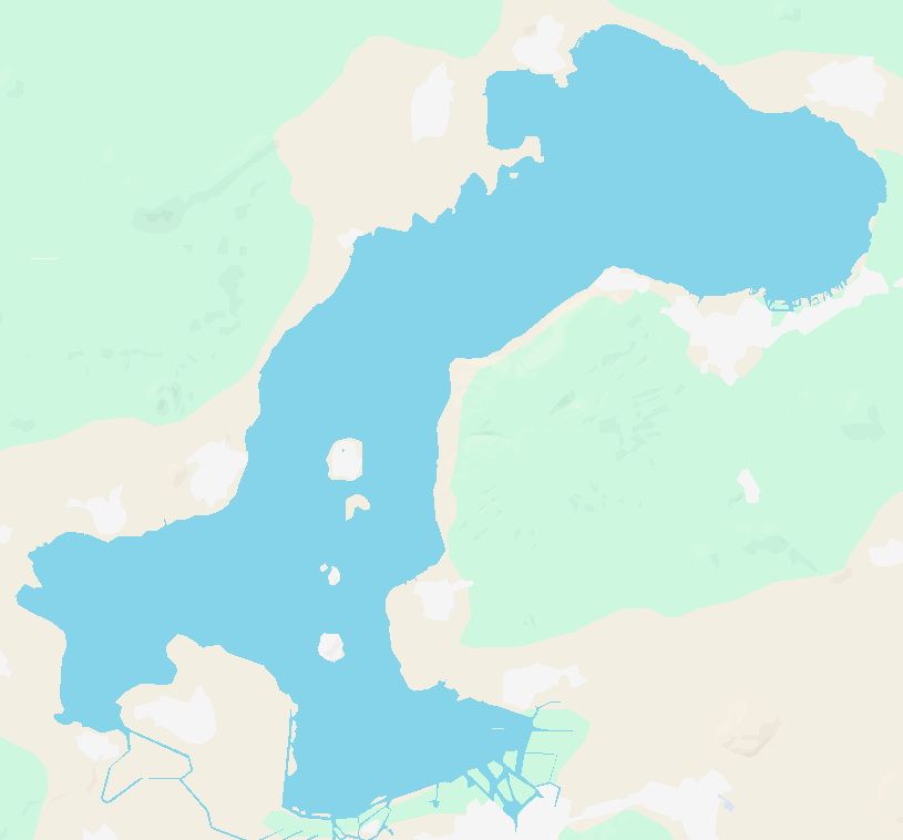
Instead of relying on idealized shapes (like circles or squares), mGFD excels at real geographic domains. We start by identifying our domain from a satellite map.
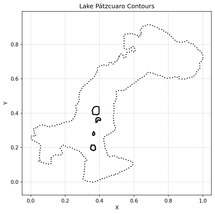
Before generating the computational point cloud, we must extract the geometric contours of the lake into a CSV file (Patzcuaro_contours.csv).
[!TIP] Visual Contour Extraction The easiest way to generate this contour file is by uploading your image to our interactive mGFD CloudGenerator Web Tool. You can manually trace the boundaries and export them directly to CSV!
| Satellite Map | Extracted Contours (CSV Plot) |
 |
 |
Step 2: Generate the Cloud (CLI)
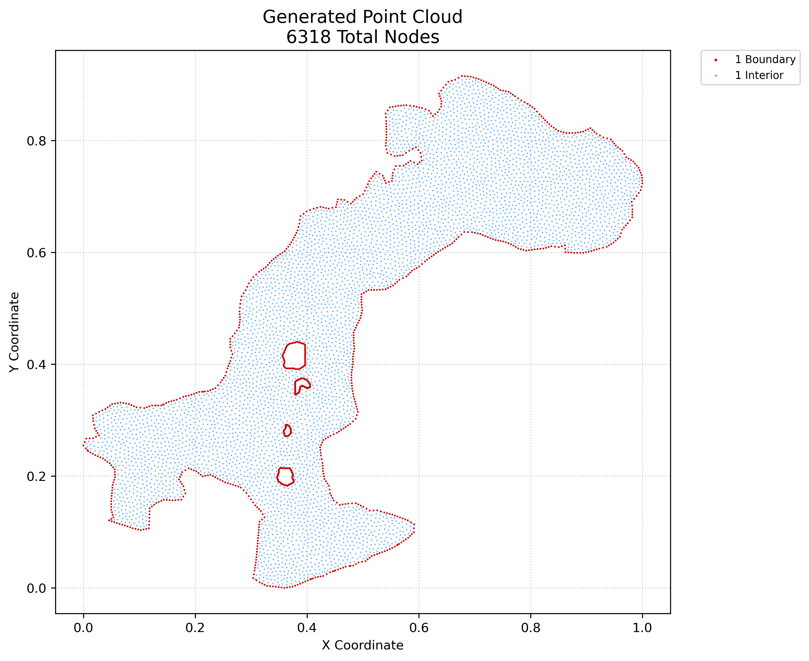
Using the mgfd-cloud CLI, we fill the interior of these extracted contours with a computationally valid, Poisson-Disk distributed point cloud:
mgfd-cloud generate --input Patzcuaro_contours.csv --output Patzcuaro_cloud.csv --method natural --density 3
Step 3: Python Solution (API)
Create a script named solve_patzcuaro.py to load your new cloud, apply the meshless solver for the Poisson equation, and render the results using the built-in visualization utilities:
import numpy as np
from mGFD.io.io import load_points
from mGFD import Stationary
from mGFD.viz.graph import plot_stationary

# 1. Load the generated point cloud
p = load_points("Patzcuaro_cloud.csv")

# 2. Define the analytical boundary condition
# Native support for Callables, Floats, or Arrays!
phi = lambda x, y: np.exp(x + y)

# 3. Define the forcing function (RHS)
f_stat = lambda x, y: 2 * np.exp(x + y)

# 4. Define the differential operator for Poisson (Laplacian)
# Vector can be 5 or 6 elements: [D, E, A, B, C, F]
L_stat = [0, 0, 2, 0, 2, 0]

# 5. Execute the solver
print("Solving Poisson Equation for Lake Pátzcuaro...")
# Returns a comprehensive SolverResult object
res = Stationary(p, phi, f_stat, operator=L_stat, linear_solver='spsolve', verbose=True)

# 6. Visualize the numerical approximation
print("Rendering plot...")
plot_stationary(p, res.solution, save=False, title='Pátzcuaro Poisson Solution', verbose=True)
Run your script, and a Matplotlib 3D window will pop up showing the surface of your solution perfectly adapted to the irregular contours of the lake!
Step 4: Visualize Results
When running batch solvers or keeping save=True, mGFD automatically exports high-quality PNGs (for stationary problems) and animated GIFs (for transient problems).
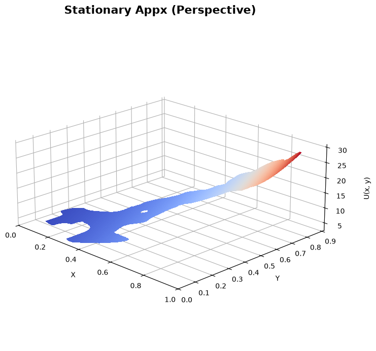
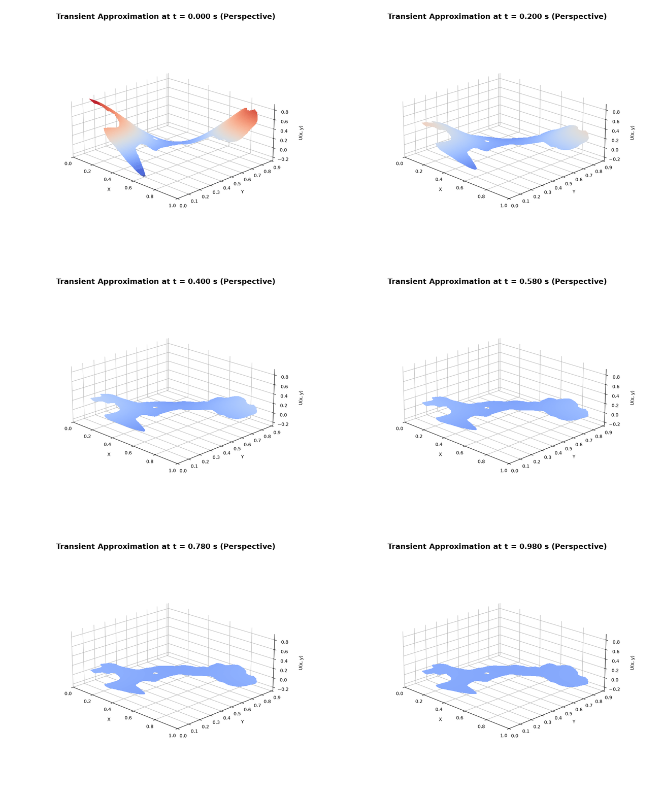
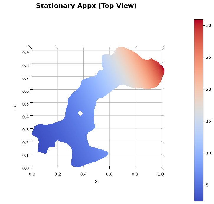
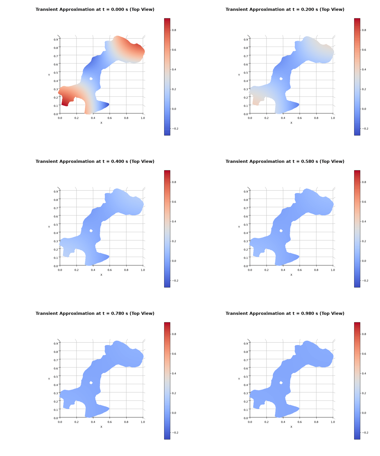
Here are the actual simulation outputs for Lake Pátzcuaro using the exact cloud generated above:
| Poisson (Stationary) | Heat (Transient) |
 |
 |
 |
 |
📚 Python API Reference
mGFD provides a clean and modular Python API located in the mGFD module. Below is an exhaustive manual of the core functions available for point cloud generation, I/O operations, PDE solving, and visualization.
1. Core Solvers (mGFD.solvers)
These functions are the mathematical heart of mGFD. They compute spatial derivatives using generalized finite differences over local neighborhoods. All solvers natively support pandas.DataFrame or numpy.ndarray as input and output.
[!TIP] mGFD Latest Features & Performance Highlights:
- ⚡ High-Performance GPU Acceleration (~90x Speedup): Replaced legacy GPU factorizations with CUDA BiCGSTAB iterative sparse solves with warm-start initial state propagation (
x0 = u_ap_gpu[:, k-1]) underdevice="cuda".- 🎬 High-Speed Animation & Graphics (~6x Speedup): Integrated
imageio-ffmpegauto-detection inmGFD.viz.graphfor multi-threaded FFmpeg GIF rendering (0.69s per animation).- ⏱️ Automatic CFL & Adaptive Time-Stepping: Automatic estimation of stable time step sizes $\Delta t$ and step counts based on Courant-Friedrichs-Lewy stability criteria (
cfl=0.5).- 🌐 Flexible Physical Time Domains: Custom time intervals $[t_{start}, t_{end}]$ via
t_span=(t0, tend).- 🎯 Independent Source & Initial/Boundary Terms: Support for independent non-homogeneous source terms $F_{source}(x, y, t)$ (
source), initial states (ic), and boundary profiles (bc).- ☁️ Adaptive Neighborhoods: KDTree C++ search algorithms dynamically build density-aware, condition-aware local stencils.
Stationary
Solves stationary problems (e.g., Poisson equation) with Dirichlet boundary conditions.
def Stationary(
    p: Union[np.ndarray, Any],
    phi: Union[Callable, np.ndarray, float, int, Any],
    f: Union[Callable, np.ndarray, float, int, Any],
    operator: np.ndarray,
    upwind: bool = False,
    vec: Optional[np.ndarray] = None,
    nvec: int = 12,
    device: str = "cpu",
    verbose: bool = True
) -> SolverResult:
TimeDerivative1
Solves first-order-in-time problems (e.g., Heat and Advection-Diffusion equations).
def TimeDerivative1(
    p: Union[np.ndarray, Any],
    f: Optional[Union[Callable, np.ndarray, float, int, Any]] = None,
    t: Optional[int] = None,
    coef: List[float] = [1.0],
    operator: Optional[np.ndarray] = None,
    implicit: bool = False,
    lam: float = 0.5,
    upwind: bool = False,
    vec: Optional[np.ndarray] = None,
    nvec: int = 12,
    device: str = "cpu",
    verbose: bool = True,
    cfl: Optional[float] = None,
    dt: Optional[float] = None,
    ic: Optional[Union[Callable, np.ndarray, float, int, Any]] = None,
    bc: Optional[Union[Callable, np.ndarray, float, int, Any]] = None,
    source: Optional[Union[Callable, np.ndarray, float, int, Any]] = None,
    t_span: Tuple[float, float] = (0.0, 1.0)
) -> SolverResult:
TimeDerivative2
Solves second-order-in-time problems (e.g., Wave equation).
def TimeDerivative2(
    p: Union[np.ndarray, Any],
    f: Optional[Union[Callable, np.ndarray, float, int, Any]] = None,
    g: Union[Callable, np.ndarray, float, int, Any] = 0.0,
    t: Optional[int] = None,
    coef: List[float] = [1.0],
    operator: Optional[np.ndarray] = None,
    upwind: bool = False,
    vec: Optional[np.ndarray] = None,
    nvec: int = 12,
    implicit: bool = True,
    lam: float = 0.25,
    device: str = "cpu",
    verbose: bool = True,
    cfl: Optional[float] = None,
    dt: Optional[float] = None,
    ic: Optional[Union[Callable, np.ndarray, float, int, Any]] = None,
    bc: Optional[Union[Callable, np.ndarray, float, int, Any]] = None,
    source: Optional[Union[Callable, np.ndarray, float, int, Any]] = None,
    t_span: Tuple[float, float] = (0.0, 1.0)
) -> SolverResult:
fd: The time derivative of the initial condition (required for computing the $u^{-1}$ ghost step).
2. Cloud Generation (mGFD.cloud_generator)
Command-Line Interface (mgfd-cloud)
The mGFD installation includes a powerful CLI to rapidly generate and reduce computational domains.
mgfd-cloud generate -i INPUT -o OUTPUT -m {natural,regular} [-d DENSITY] [--inside-regions]

mgfd-cloud reduce -i INPUT -o OUTPUT -m MULTIPLIER
generate: Fills a boundary contour with points.-i/--input: Path to the boundary CSV file.-o/--output: Path for the generated cloud CSV.-m/--method: Usenatural(Poisson-Disk) orregular(Grid).-d/--density: Density multiplier. Higher values create denser, tighter clouds.--inside-regions: If present, internal closed boundaries are treated as solid islands (holes in the domain).
reduce: Reduces the density of an existing cloud.-m/--multiplier: Scaling factor to space out points.
While the CLI (mgfd-cloud) is the easiest way to generate domains, you can invoke the generation directly via Python.
generate_cloud_natural / generate_cloud_regular
Generates an unstructured (Poisson-Disk) or regular (Grid) point cloud inside a contour.
def generate_cloud_natural(
    csv_file: str,
    output_file: str,
    inside_regions: bool = False,
    verbose: bool = False
)

def generate_cloud_regular(
    csv_file: str,
    output_file: str,
    inside_regions: bool = False,
    verbose: bool = False
)
csv_file: Path to the input contour CSV file.output_file: Path where the generated cloud CSV will be saved.inside_regions: IfTrue, interprets internal closed contours as solid islands (holes in the domain).
reduce_points_by_region
Reduces the point density of an existing cloud by a scaling factor.
def reduce_points_by_region(
    input_csv: str,
    output_csv: str,
    multiplier: int = 2
) -> Optional[List[Dict[str, Any]]]
multiplier: A scaling factor for the distance between nodes. A multiplier of2significantly reduces the number of points.
3. I/O Operations (mGFD.io.io)
load_points
def load_points(
    file_path: str,
    verbose: bool = False
) -> np.ndarray
- Reads a CSV file containing
x, y, flagdata and returns it as a standardized(m, 3)NumPy array ready for the solvers.
export_stationary_vtk / export_transient_vtk (mGFD.io.export_vtk)
Exports the numerical solutions directly to VTK format using PyVista, perfectly structured for advanced 3D analysis in Paraview.
def export_stationary_vtk(
    p: np.ndarray,
    u_ap: np.ndarray,
    out_dir: str,
    basename: str = "Stationary_Solution",
    cloud_path: Optional[str] = None
) -> None

def export_transient_vtk(
    p: np.ndarray,
    u_ap: np.ndarray,
    t: int,
    T: np.ndarray,
    out_dir: str,
    basename: str = "Transient_Solution",
    cloud_path: Optional[str] = None
) -> None
u_ap: The computed numerical approximation array (or matrix for transients).out_dir: Directory where the.vtkfiles will be saved.cloud_path: (Optional) Passing the original cloud path allowsmGFDto automatically locate and use the cached triangulation to build the PyVista mesh instantly.
4. Visualization Utilities (mGFD.viz.graph)
plot_stationary
def plot_stationary(
    p: np.ndarray,
    u: np.ndarray,
    save: bool = False,
    nom: str = '',
    title: str = 'Solution',
    verbose: bool = True
) -> None
- Renders a 3D scatter surface of the solution over the point cloud. If
save=True, it exports.pngsnapshots to thenompath.
plot_transient
def plot_transient(
    p: np.ndarray,
    u: np.ndarray,
    save: bool = False,
    nom: str = '',
    title: str = 'Solution',
    verbose: bool = True
) -> None
u(m x t): A matrix containing the solution at each node for every time step.- Renders a 3D Matplotlib animation over time. If
save=True, it exports an animated.gifto thenompath.
5. Core Utilities & Triangulations (mGFD.core.utils)
Because mGFD is a strictly meshless numerical method, the PDE solvers operate entirely on unstructured points and local distance-based neighborhoods (stencils). Meshes/triangles are never used during the numerical solution.
However, rendering 3D surfaces in Matplotlib and exporting meshes to Paraview (VTK) mathematically requires a triangulation to color the faces between points.
get_valid_triangulation
def get_valid_triangulation(p: np.ndarray, nom: Optional[str] = None) -> Optional[np.ndarray]
- What it does: Computes a constrained Delaunay triangulation of the point cloud, aggressively filtering out triangles that fall outside concave boundaries or inside holes (islands).
- Caching system: Computing Delaunay simplices on large clouds is extremely expensive. When
mGFDcomputes a valid triangulation, it automatically caches the resulting simplices into a_triangulation.csvfile next to your original cloud. Subsequent calls to plotting or VTK exports will load this cache, saving massive amounts of computation time.
⚡ High Performance & GPU Acceleration Guide
When scaling up to massive geographic regions (hundreds of thousands of points) or ultra-dense domains, memory (RAM) and computation time become the primary bottlenecks. mGFD introduces two powerful paradigms to solve PDEs on these massive datasets.
1. Matrix-Free Operations (CPU Optimization)
Standard linear algebraic solvers construct a massive $M \times M$ sparse matrix. Even when sparse, storing this structure for 1,000,000 points consumes gigabytes of memory.
By setting matrix_free=True, mGFD completely bypasses the creation of the global Sparse Matrix. Instead, it utilizes Numba JIT-compiled parallel closures to compute matrix-vector multiplications ($K \cdot x$) directly on the fly using the point cloud geometry.
Best for: Systems with limited RAM but decent multi-core processors.
Available Solvers: Requires an iterative Krylov subspace solver (e.g., linear_solver="bicgstab" or "gmres").
# Extremely RAM-efficient solve on the CPU
res = Stationary(
    p, phi, f_stat, operator=L_stat,
    linear_solver="bicgstab",
    matrix_free=True,
    device="cpu"
)
2. GPU Acceleration (NVIDIA CUDA)
If you have an NVIDIA GPU and installed cupy, you can offload the entire linear algebra resolution to VRAM. mGFD handles the memory transfers seamlessly.
[!WARNING] CPU vs GPU Performance Paradigms GPUs are designed for massive parallelism, while CPUs excel at sequential logic.
- Use
device="cpu"for small-to-medium clouds (e.g. < 50,000 nodes), especially when using implicit methods (implicit=True) which require sequential triangular solves (spsolve) or iterative logic (bicgstab). The CPU will often be much faster due to low overhead.- Use
device="cuda"ONLY for massive point clouds where the CPU runs out of memory, OR when using Explicit Methods (implicit=False) which map perfectly to the GPU's parallel architecture.
Best for: Massive speedups on large domains if you have the VRAM to hold the sparse matrix, or when running explicit time integration.
Available Solvers: Works exceptionally well with direct solvers (linear_solver="spsolve") and iterative solvers.
# Extremely fast solve on the GPU
res = Stationary(
    p, phi, f_stat, operator=L_stat,
    linear_solver="spsolve",
    device="cuda"
)
(Note: matrix_free=True cannot currently be combined with device="cuda", as Matrix-Free relies on CPU Numba multithreading).
3. Preconditioners for Iterative Solvers
When using iterative solvers (bicgstab, gmres) on highly irregular clouds, the matrix condition number can degrade, leading to slow convergence or failure. mGFD provides built-in preconditioners to rescue these situations:
- Jacobi (
preconditioner="jacobi"): Extremely fast, diagonal scaling. Works well for bothmatrix_freeCPU andcudaGPU solves. - Incomplete LU (
preconditioner="ilu"): Powerful factorization technique. Recommended for ill-conditioned matrices on CPU (matrix_free=False), and fully supported on GPU (cuda).
# The ultimate robust solver setup for tough hyperbolic problems on GPU:
res = TimeDerivative2(
    p, f_func, g_func, t_steps, [c], operator=L_wave,
    linear_solver="gmres",
    preconditioner="ilu",
    device="cuda",
    implicit=True
)
🔬 Research & Datasets
Looking for the mathematical formulation, real-world geographic lake datasets (Lake Patzcuaro, Caspian Sea, etc.), or reproducible benchmarking scripts?
👉 Explore the Research Laboratory (/research/README.md)
The research/ directory contains our complete academic suite, including experimental data, geographic boundary files, VTK results, and the exact theoretical explanations associated with our scientific publications.
🏗️ Repository Structure
Understanding the layout of this project is helpful if you want to contribute or explore the underlying math:
mGFD/
├── docs/                     # Media assets for the README (images, gifs)
├── src/mGFD/                 # The core Python library (uploaded to PyPI)
│   ├── cloud_generator/      # PDE domain creation (natural, regular, etc.)
│   ├── spatial/              # Spatial discretization: KDTree neighbors, stencils
│   ├── io/                   # CSV and VTK import/export operations
│   ├── solvers/              # The high-level PDE solvers (with private _backends)
│   ├── utils/                # Pandas/Xarray adapters and helper functions
│   └── viz/                  # Matplotlib 3D and 2D rendering
├── research/                 # The academic reproducible suite
│   ├── codes/                # Batch benchmarking scripts (e.g. main.py)
│   ├── data/                 # Geographic boundaries (CSV files)
│   ├── results/              # Output GIFs, VTKs, PNGs, and metrics
│   └── README.md             # Detailed mathematical foundations
└── tests/                    # CI/CD Unit and Integration tests
🤝 Contributing & Citation
Contributing
We welcome contributions from the scientific and open-source community!
- Fork the repository.
- Clone your fork locally and create a new feature branch (
git checkout -b feature-new-solver). - Develop your feature, ensuring all code strictly adheres to our PEP-8 standard (especially the inline
#alignment at column 136). - Test your code (we run a comprehensive CI suite via GitHub Actions).
- Open a Pull Request!
For major changes, please open an issue first to discuss what you would like to change.
Citation
This project is open-sourced under the MIT License.
If you use this library or the core mathematical methodology in your research, please cite our reference paper:
@article{tinoco2025mgfd,
  title={mGFD: A meshless generalized finite difference method},
  author={Tinoco-Guerrero, Gerardo and Domínguez-Mota, Francisco Javier and Guzmán-Torres, José Alberto and Pedraza-Jiménez, Gabriela and Tinoco-Ruiz, José Gerardo},
  journal={Computers & Mathematics with Applications},
  volume={195},
  pages={396--418},
  year={2025},
  publisher={Elsevier},
  doi={10.1016/j.camwa.2025.07.034}
}
Developed for the advancement of meshless numerical methods and scientific computing.
Dr. Gerardo Tinoco-Guerrero
Dr. Francisco Javier Domínguez-Mota
Dr. José Alberto Guzmán-Torres
Universidad Michoacana de San Nicolás de Hidalgo
gerardo.tinoco@umich.mx
Report a Bug | Contact Author
1 maintainer

Download files
Download the file for your platform. If you're not sure which to choose, learn more about installing packages.
Source Distribution
Built Distribution
Filter files by name, interpreter, ABI, and platform.
If you're not sure about the file name format, learn more about wheel file names.
Copy a direct link to the current filters
File details
Details for the file mgfd-0.11.1.tar.gz.
File metadata
- Download URL: mgfd-0.11.1.tar.gz
- Upload date:
- Size: 126.7 kB
- Tags: Source
- Uploaded using Trusted Publishing? No
- Uploaded via:
twine/7.0.0 CPython/3.13.7
File hashes
| Algorithm | Hash digest | |
|---|---|---|
| SHA256 |
d255a4ac5d4fbb5df6b3f16afdc53aa23b9982f9c3f2e375cd8273cc00a09be8
|
|
| MD5 |
d6018568e4c825e7f4c114323800455c
|
|
| BLAKE2b-256 |
7a8c4ca16d1caab8d8a71d0f88c89f4fcefbd5dcfefa05707aed2ae44e1742d5
|
File details
Details for the file mgfd-0.11.1-py3-none-any.whl.
File metadata
- Download URL: mgfd-0.11.1-py3-none-any.whl
- Upload date:
- Size: 162.3 kB
- Tags: Python 3
- Uploaded using Trusted Publishing? No
- Uploaded via:
twine/7.0.0 CPython/3.13.7
File hashes
| Algorithm | Hash digest | |
|---|---|---|
| SHA256 |
e7debf3f7c8a13e2638e9d0d2534e91bd70dcdb88fab651652dbb2d8220cc224
|
|
| MD5 |
d22b84dc68855012098ebce18405eb30
|
|
| BLAKE2b-256 |
838c1fed2c53d843fbacab33fe1f002cf99473f159d046e95477ab126392be0d
|














