
Object-oriented machine vision for Python.

Project description
Machine Vision Toolbox for Python

A high-productivity framework for computer vision research and education.



GitHub • Wiki • Changelog • Installation
Status & Ecosystem







Powered by




Synopsis
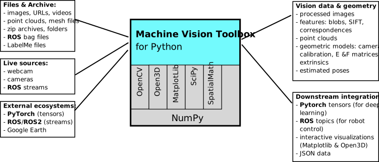
A unified, object-oriented Python API that bridges the gap between raw pixels and high-level spatial reasoning by harmonizing a 'best-of-breed' foundation of NumPy, OpenCV, and Open3D. It bridges the gap between raw pixel manipulation and high-level spatial reasoning and robotics.
🚀 Key components
-
The power object:
Imageis a single class wrapping 200+ methods. It handles everything from monadic/dyadic ops and edge detection to advanced feature extraction (blobs, lines, and point features) with full operator overloading. -
Advanced Camera Modeling: Comprehensive support for Central (perspective), Fisheye, Catadioptric, and Spherical camera geometries.
-
Spatial AI Integration: Native compatibility with the Spatial Math Toolbox and seamless "play" with PyTorch and ROS.
-
High-Level 3D Vision: Sophisticated wrappers for Open3D, including multiview geometry, camera calibration, stereo vision, and bundle adjustment.
🛠 Why MVTB?
-
Expressive Method Chaining: Build complex pipelines in a single, readable line:
Image.Read("monalisa.png").convolve(Kernel.Gauss(4)).disp() -
"Sanity-Preserving" OpenCV Wrappers: We handle the "gnarly" bits of OpenCV for you—automatically managing BGR-to-RGB conversions and float32 scaling so you can focus on the vision, not the boilerplate.
-
NumPy-Native: Every image is an encapsulated NumPy array, meaning you have zero-overhead access to the entire Python scientific stack.
-
2026 Ready: Optimized for modern workflows, including JupyterLite for zero-install browser demos and VS Code integration.
Quick start
Install a snapshot from PyPI
% pip install machinevision-toolbox-python
Install locally with help from the detailed installation guide.
Or skip setup and run the browser-based JupyterLite examples.
Examples
Reading and display an image
from machinevisiontoolbox import Image
mona = Image.Read("monalisa.png")
mona.disp()
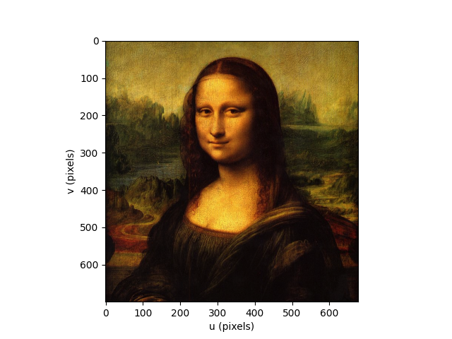
Images can also be returned by iterators that operate over folders, zip files, local cameras, web cameras and video files.
Simple image processing
The toolbox supports many operations on images such as 2D filtering, edge detection, mathematical morphology, colorspace conversion, padding, cropping, resizing, rotation and warping.
mona.smooth(sigma=5).disp()
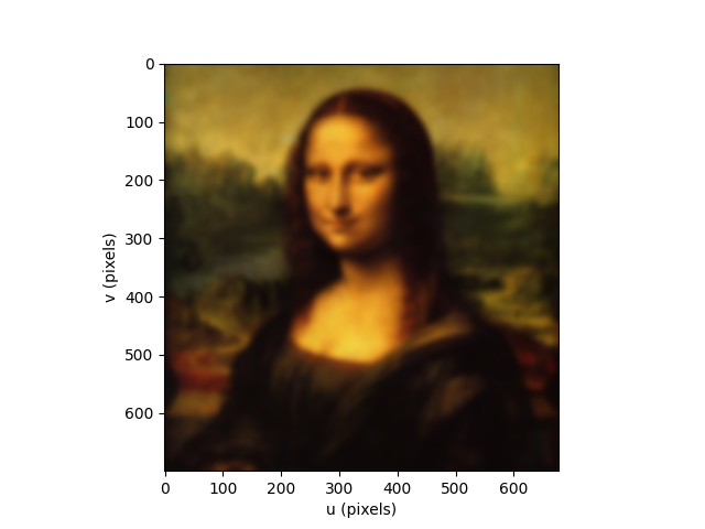
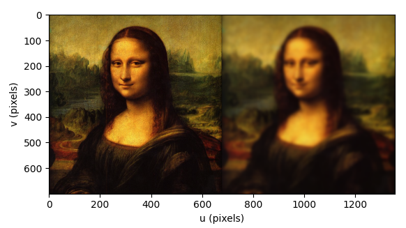
There are also many functions that operate on pairs of image. All the arithmetic operators are overloaded, and there are methods to combine images in more complex ways. Multiple images can be stacked horizontal, vertically or tiled in a 2D grid. For example, we could display the original and smoothed images side by side
Image.Hstack([mona, mona.smooth(sigma=5)]).disp()
where Hstack is a class method that creates a new image by stacking the
images from its argument, an image sequence, horizontally.
Binary blobs
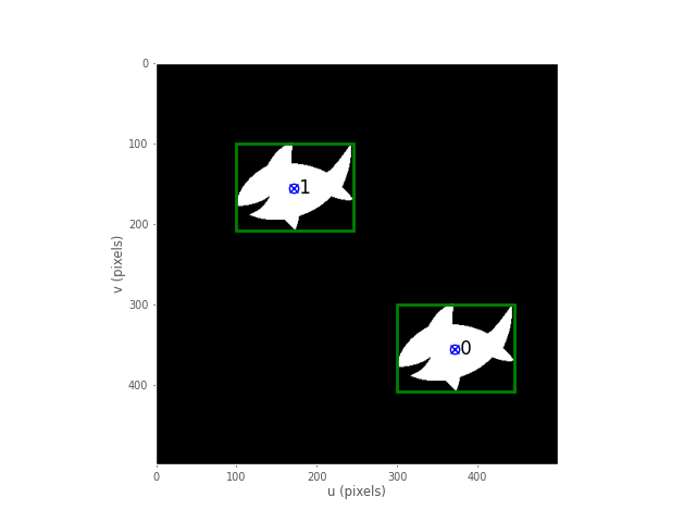
A common problem in robotic vision is to extract features from the image, to describe the position, size, shape and orientation of objects in the scene. For simple binary scenes blob features are commonly used.
im = Image.Read("shark2.png")   # read a binary image of two sharks
im.disp();   # display it with interactive viewing tool
blobs = im.blobs()  # find all the white blobs
print(blobs)

	┌───┬────────┬──────────────┬──────────┬───────┬───────┬─────────────┬────────┬────────┐
	│id │ parent │     centroid │     area │ touch │ perim │ circularity │ orient │ aspect │
	├───┼────────┼──────────────┼──────────┼───────┼───────┼─────────────┼────────┼────────┤
	│ 0 │     -1 │ 371.2, 355.2 │ 7.59e+03 │ False │ 557.6 │       0.341 │  82.9° │  0.976 │
	│ 1 │     -1 │ 171.2, 155.2 │ 7.59e+03 │ False │ 557.6 │       0.341 │  82.9° │  0.976 │
	└───┴────────┴──────────────┴──────────┴───────┴───────┴─────────────┴────────┴────────┘
where blobs is a list-like object and each element describes a blob in the scene. The element's attributes describe various parameters of the object, and methods can be used to overlay graphics such as bounding boxes and centroids
blobs.plot_box(color="g", linewidth=2)  # put a green bounding box on each blob
blobs.plot_centroid(label=True)  # put a circle+cross on the centroid of each blob
plt.show(block=True)  # display the result
Binary blob hierarchy
A more complex image is
im = Image.Read("multiblobs.png")
im.disp()
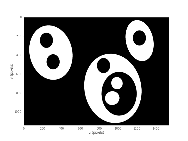
and we see that some blobs are contained within other blobs. The results in tabular form
blobs  = im.blobs()
print(blobs)
	┌───┬────────┬───────────────┬──────────┬───────┬────────┬─────────────┬────────┬────────┐
	│id │ parent │      centroid │     area │ touch │  perim │ circularity │ orient │ aspect │
	├───┼────────┼───────────────┼──────────┼───────┼────────┼─────────────┼────────┼────────┤
	│ 0 │      1 │  898.8, 725.3 │ 1.65e+05 │ False │ 2220.0 │       0.467 │  86.7° │  0.754 │
	│ 1 │      2 │ 1025.0, 813.7 │ 1.06e+05 │ False │ 1387.9 │       0.769 │ -88.9° │  0.739 │
	│ 2 │     -1 │  938.1, 855.2 │ 1.72e+04 │ False │  490.7 │       1.001 │  88.7° │  0.862 │
	│ 3 │     -1 │  988.1, 697.2 │ 1.21e+04 │ False │  412.5 │       0.994 │ -87.8° │  0.809 │
	│ 4 │     -1 │  846.0, 511.7 │ 1.75e+04 │ False │  496.9 │       0.992 │ -90.0° │  0.778 │
	│ 5 │      6 │  291.7, 377.8 │  1.7e+05 │ False │ 1712.6 │       0.810 │ -85.3° │  0.767 │
	│ 6 │     -1 │  312.7, 472.1 │ 1.75e+04 │ False │  495.5 │       0.997 │ -89.9° │  0.777 │
	│ 7 │     -1 │  241.9, 245.0 │ 1.75e+04 │ False │  496.9 │       0.992 │ -90.0° │  0.777 │
	│ 8 │      9 │ 1228.0, 254.3 │ 8.14e+04 │ False │ 1215.2 │       0.771 │ -77.2° │  0.713 │
	│ 9 │     -1 │ 1225.2, 220.0 │ 1.75e+04 │ False │  496.9 │       0.992 │ -90.0° │  0.777 │
	└───┴────────┴───────────────┴──────────┴───────┴────────┴─────────────┴────────┴────────┘
We can display a label image, where the value of each pixel is the label of the blob that the pixel
belongs to, the id attribute
labels = blobs.label_image()
labels.disp(colormap="viridis", ncolors=len(blobs), colorbar=dict(shrink=0.8, aspect=20*0.8))
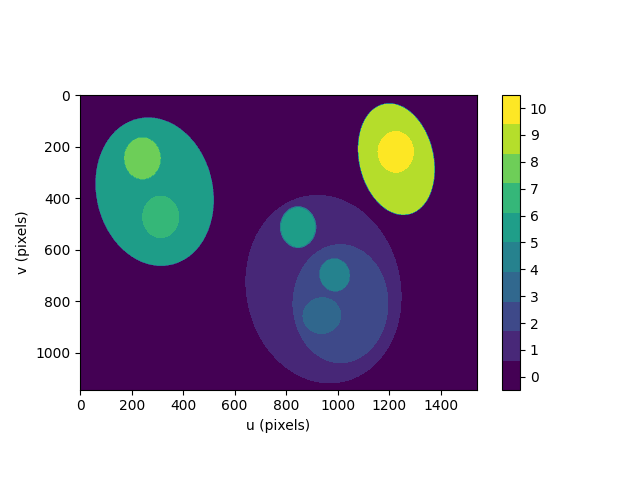
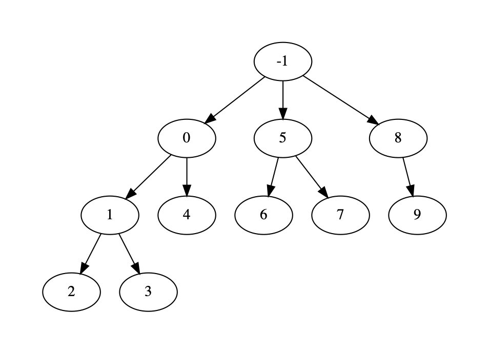
We can also think of the blobs forming a hiearchy and that relationship is reflected in the parent and children attributes of the blobs.
We can also express it as a directed graph
blobs.dotfile(show=True)
Camera modelling
from machinevisiontoolbox import CentralCamera
cam = CentralCamera(f=0.015, rho=10e-6, imagesize=[1280, 1024], pp=[640, 512], name="mycamera")
print(cam)
           Name: mycamera [CentralCamera]
     pixel size: 1e-05 x 1e-05
     image size: 1280 x 1024
           pose: t = 0, 0, 0; rpy/yxz = 0°, 0°, 0°
   principal pt: [     640      512]
   focal length: [   0.015    0.015]
and its intrinsic parameters are
print(cam.K)
	[[1.50e+03 0.00e+00 6.40e+02]
	 [0.00e+00 1.50e+03 5.12e+02]
	 [0.00e+00 0.00e+00 1.00e+00]]
We can define an arbitrary point in the world
P = [0.3, 0.4, 3.0]
and then project it into the camera
p = cam.project(P)
print(p)
	[790. 712.]
which is the corresponding coordinate in pixels. If we shift the camera slightly the image plane coordinate will also change
p = cam.project(P, T=SE3(0.1, 0, 0) )
print(p)
[740. 712.]
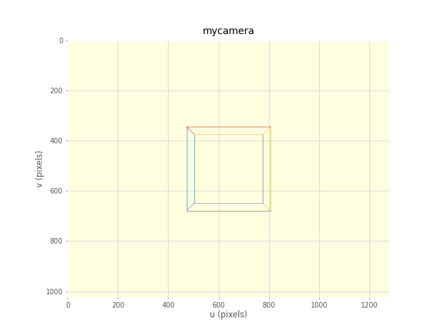
We can define an edge-based cube model and project it into the camera's image plane
from spatialmath import SE3
X, Y, Z = mkcube(0.2, pose=SE3(0, 0, 1), edge=True)
cam.plot_wireframe(X, Y, Z)
Color space
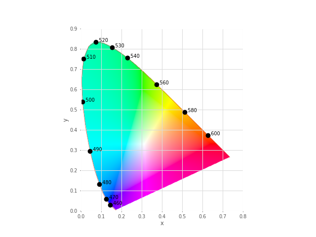
Plot the CIE chromaticity space
plot_chromaticity_diagram("xy");
plot_spectral_locus("xy")
Load the spectrum of sunlight at the Earth's surface and compute the CIE xy chromaticity coordinates
nm = 1e-9
lam = np.linspace(400, 701, 5) * nm # visible light
sun_at_ground = loadspectrum(lam, "solar")
xy = lambda2xy(lambda, sun_at_ground)
print(xy)
	[[0.33272798 0.3454013 ]]
print(colorname(xy, "xy"))
	khaki
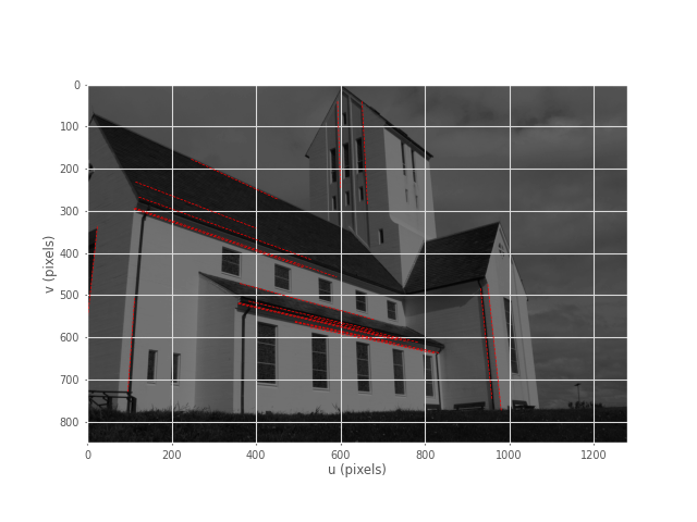
Hough transform
im = Image.Read("church.png", mono=True)
edges = im.canny()
h = edges.Hough()
lines = h.lines_p(100, minlinelength=200, maxlinegap=5, seed=0)

im.disp(darken=True)
h.plot_lines(lines, "r--")
SURF features
We load two images and compute a set of SURF features for each
view1 = Image.Read("eiffel-1.png", mono=True)
view2 = Image.Read("eiffel-2.png", mono=True)
sf1 = view1.SIFT()
sf2 = view2.SIFT()
We can match features between images based purely on the similarity of the features, and display the correspondences found
matches = sf1.match(sf2)
print(matches)
813 matches
matches[1:5].table()
┌──┬────────┬──────────┬─────────────────┬────────────────┐
│# │ inlier │ strength │              p1 │             p2 │
├──┼────────┼──────────┼─────────────────┼────────────────┤
│0 │        │     26.4 │ (1118.6, 178.8) │ (952.5, 418.0) │
│1 │        │     28.2 │ (820.6, 519.1)  │ (708.1, 701.6) │
│2 │        │     29.6 │ (801.1, 632.4)  │ (694.1, 800.3) │
│3 │        │     32.4 │ (746.0, 153.1)  │ (644.5, 392.2) │
└──┴────────┴──────────┴─────────────────┴────────────────┘
where we have displayed the feature coordinates for four correspondences.
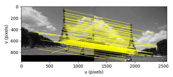
We can also display the correspondences graphically
matches.subset(100).plot("w")
in this case, a subset of 100/813 of the correspondences.
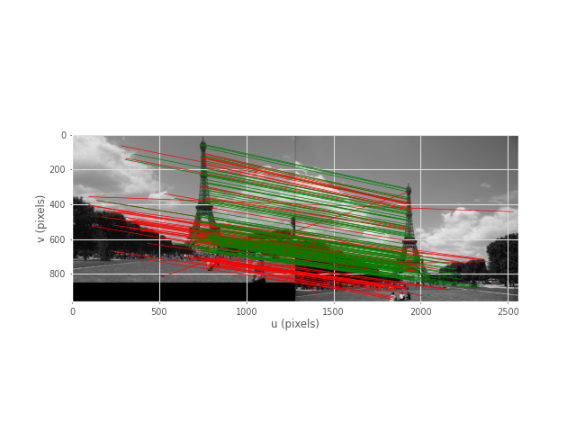
Clearly there are some bad matches here, but we we can use RANSAC and the epipolar constraint implied by the fundamental matrix to estimate the fundamental matrix and classify correspondences as inliers or outliers
F, resid = matches.estimate(CentralCamera.points2F, method="ransac", confidence=0.99, seed=0)
print(F)
array([[1.033e-08, -3.799e-06, 0.002678],
       [3.668e-06, 1.217e-07, -0.004033],
       [-0.00319, 0.003436,        1]])
print(resid)
0.0405

Image.Hstack((view1, view2)).disp()
matches.inliers.subset(100).plot("g", ax=plt.gca())
matches.outliers.subset(100).plot("r", ax=plt.gca())
where green lines show correct correspondences (inliers) and red lines show bad correspondences (outliers)
Ecosystem
The Toolbox plays nicely with other parts of the robotics and machinevision ecosystem.
History
This package can be considered as a Python version of the Machine Vision Toolbox for MATLAB. That Toolbox, now quite old, is a collection of MATLAB functions and classes that supported the first two editions of the Robotics, Vision & Control book. It is a somewhat eclectic collection reflecting my personal interest in areas of photometry, photogrammetry, colorimetry. It includes over 100 functions spanning operations such as image file reading and writing, acquisition, display, filtering, blob, point and line feature extraction, mathematical morphology, homographies, visual Jacobians, camera calibration and color space conversion.
This Python version differs in using an object to encapsulate the pixel data and image metadata, rather than just a native object holding pixel data. The many functions become methods of the image object which reduces namespace pollutions, and allows the easy expression of sequential operations using "dot chaining".
Acknowledgement
The first version was built by Dorian Tsai during 2020-21, and based on the MATLAB version. That work was funded by an Australian University Teacher of the year award (2017) to Peter Corke.
Release history Release notifications | RSS feed


Download files
Download the file for your platform. If you're not sure which to choose, learn more about installing packages.
Source Distribution
Built Distribution
Filter files by name, interpreter, ABI, and platform.
If you're not sure about the file name format, learn more about wheel file names.
Copy a direct link to the current filters
File details
Details for the file machinevision_toolbox_python-2.0.1.tar.gz.
File metadata
- Download URL: machinevision_toolbox_python-2.0.1.tar.gz
- Upload date:
- Size: 6.0 MB
- Tags: Source
- Uploaded using Trusted Publishing? No
- Uploaded via: twine/6.2.0 CPython/3.12.8
File hashes
| Algorithm | Hash digest | |
|---|---|---|
| SHA256 |
aaa26071787c85b907ef1137c2191996f1c69da2f42d0dff121d9f355e096c9f
|
|
| MD5 |
dda472d9a285d77c2093eea49c1f3848
|
|
| BLAKE2b-256 |
9d4a0b80f0bc7235fb51aa0edbad482b81a0be6b8a31dc40b2472779b6c8691f
|
File details
Details for the file machinevision_toolbox_python-2.0.1-py3-none-any.whl.
File metadata
- Download URL: machinevision_toolbox_python-2.0.1-py3-none-any.whl
- Upload date:
- Size: 455.4 kB
- Tags: Python 3
- Uploaded using Trusted Publishing? No
- Uploaded via: twine/6.2.0 CPython/3.12.8
File hashes
| Algorithm | Hash digest | |
|---|---|---|
| SHA256 |
fd8fb3248471afc925d747c907d31cdc6262fc9dcef38ea67269510611d6a19e
|
|
| MD5 |
bfef10b4f8d04fce04f6daee62ca7d52
|
|
| BLAKE2b-256 |
5a20fb9f94d4f46463c172f140eb7d0c539e04bfde33a13c8d2f04a1e69ce512
|






