
Magnus







Code to compute neutrino oscillation probabilities between an arbitrary number of flavors, for any given Hamiltonian, time-dependent or -independent.
How do I say that? Just like the name Magnus — the Greek letter ν (nu), the neutrino's symbol, simply stands in for the "nu" syllable. (And since most of this package was written while the author was based in Denmark, you are equally welcome to say it the Danish way.)
How it works. Magnus computes the neutrino evolution operator via the Magnus expansion: instead of integrating the Schrödinger equation step by step, it exponentiates truncated time-ordered integrals of the Hamiltonian over a chain of position slabs. Any truncation of the Magnus series lives in the Lie algebra, so the resulting evolution operator is exactly unitary by construction — probabilities are non-negative and sum to one at machine precision, at any accuracy setting. The full derivation, term by term, is in the mathematical method page of the documentation.
Installation
pip install magnuspy
Python 3.10 or newer. The distribution is called magnuspy on PyPI because
plain magnus was already taken by an unrelated project — but the import
package is magnus:
import magnus.oscprob as oscprob
From a checkout, pip install -e . instead; add '.[test]' for the test
extras. See the installation
page for the optional
extras and the full dependency list.
What you can compute
Every figure below is produced by a notebook in notebooks/, and the link under each one goes to the code that drew it — the images are lifted out of the executed notebooks rather than plotted separately, so what you see is what that notebook produced. The documentation collects the same material, with runnable snippets, on its numerical recipes page.
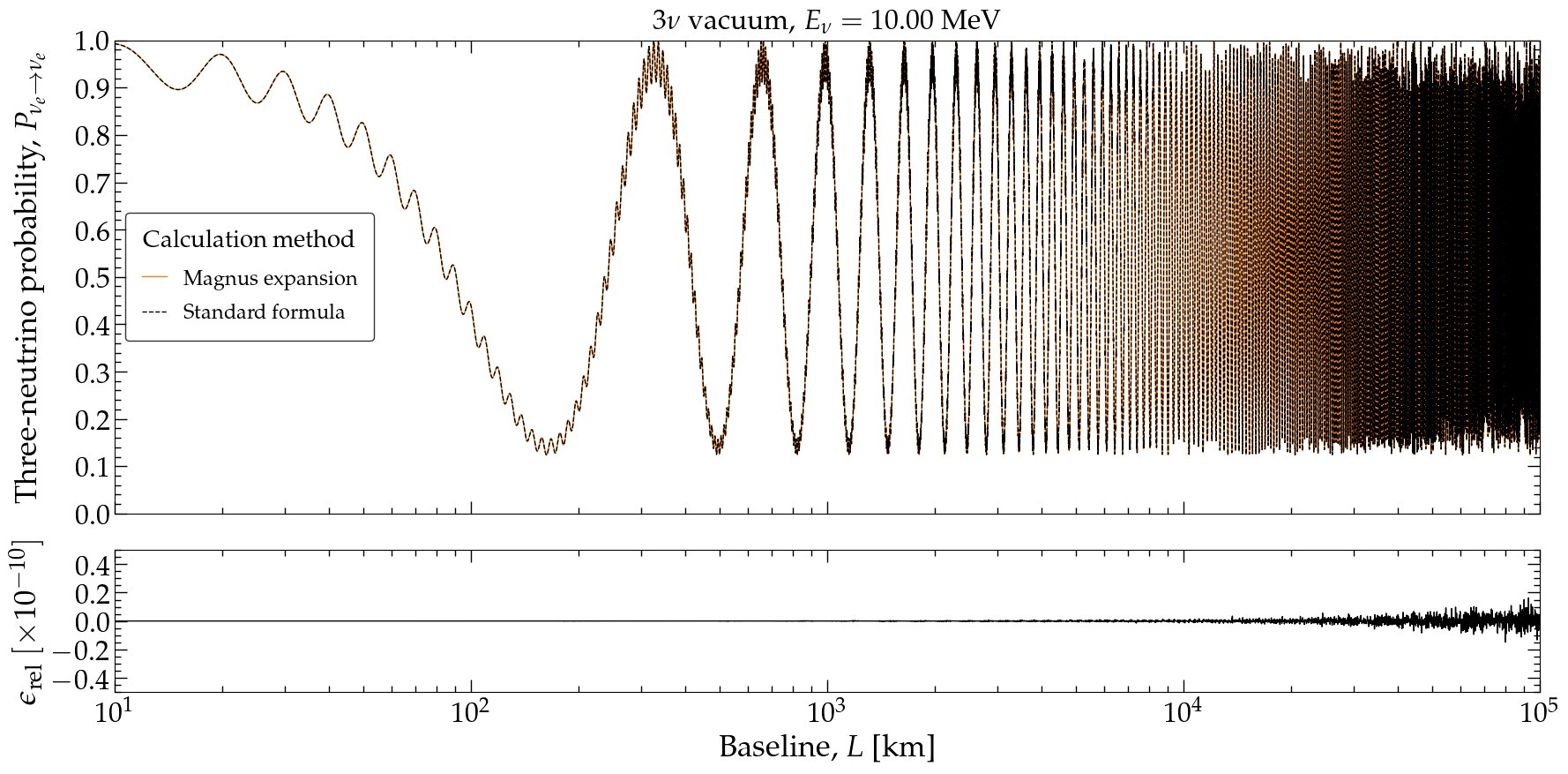 Oscillation probabilities against baseline or energy, for two to five flavors, in vacuum and in matter. notebook 03 |
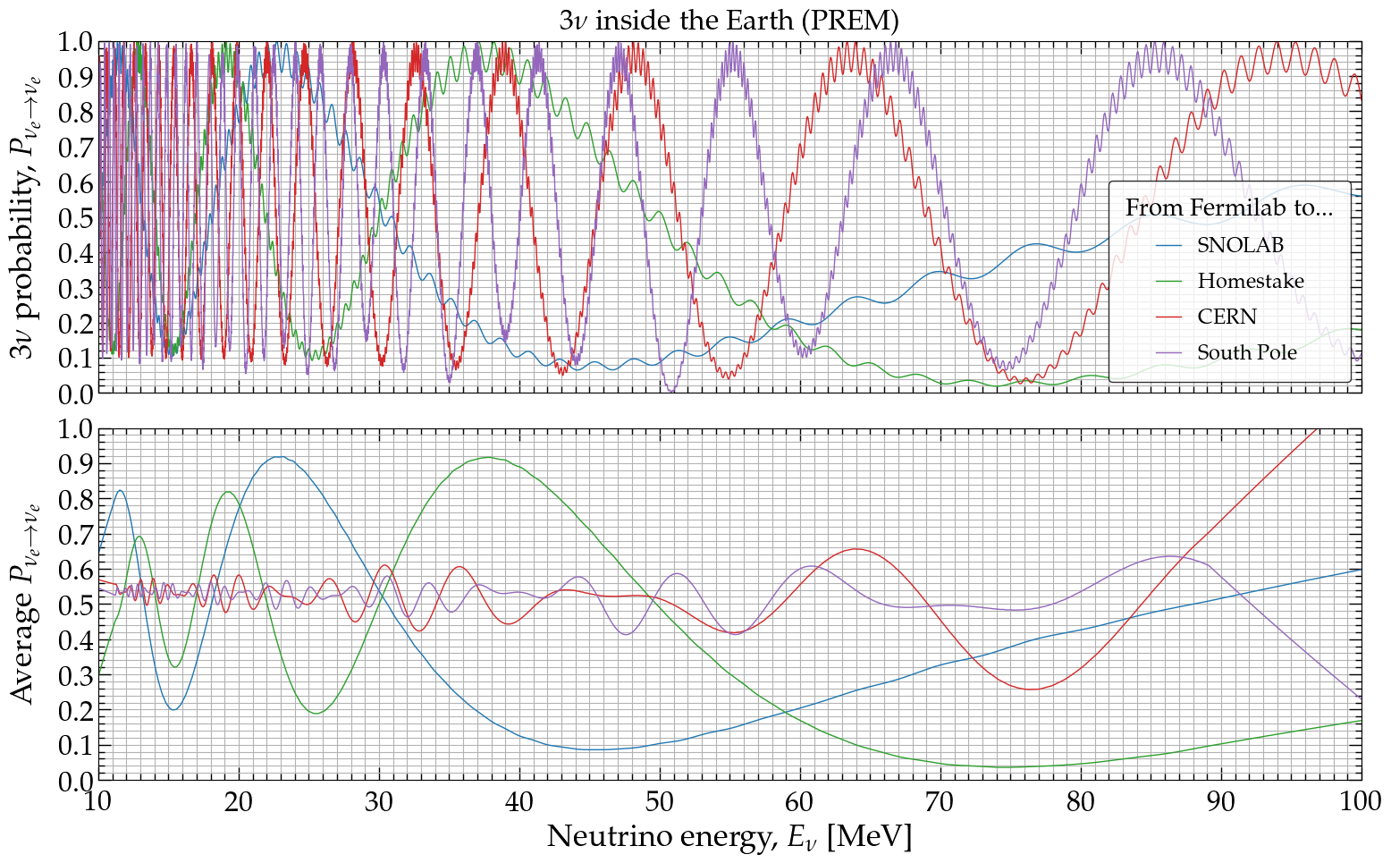 Between two points on the Earth's surface — Fermilab to SNOLAB, Homestake, CERN and the South Pole, through PREM. notebook 04 |
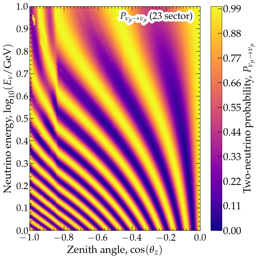 Oscillograms across zenith angle and energy, in a single call. notebook 06 |
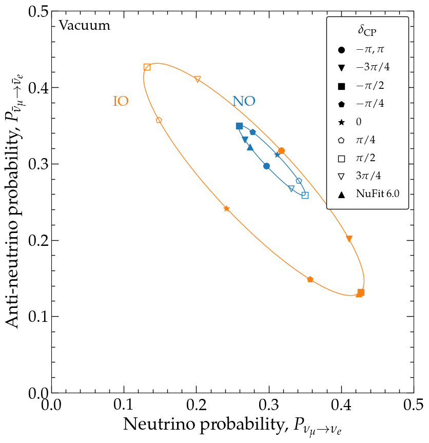 CP violation, as bi-probability ellipses traced by the CP phase. notebook 05 |
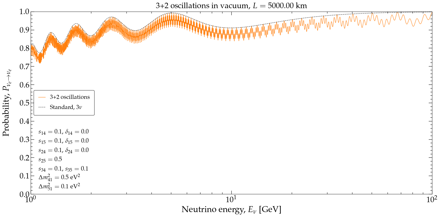 Five flavors: a 3+2 sterile spectrum, its fast oscillation filling the three-flavor envelope. notebook 07 |
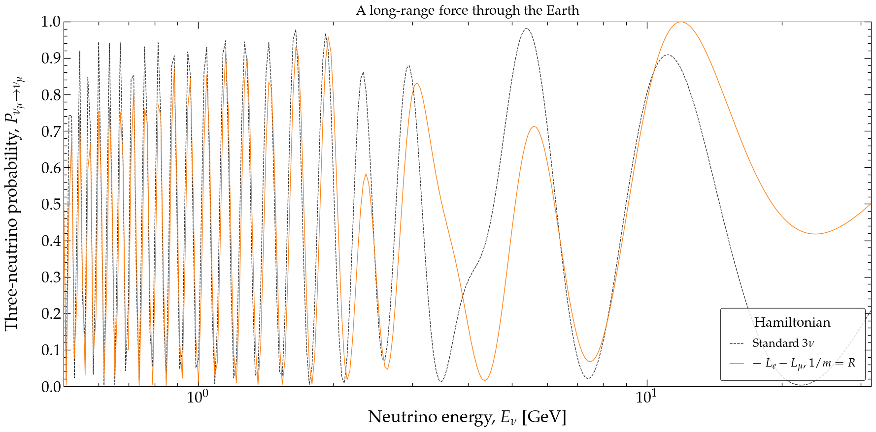 A Hamiltonian of your own — here a long-range $L_e - L_\mu$ force through the Earth, against the standard curve. notebook 19 |
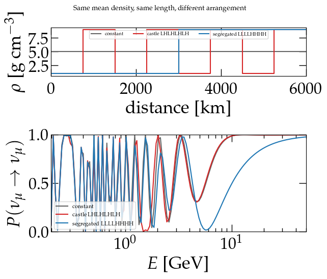 Arrangement beats the mean: the same average density and the same path length, ordered differently, give different probabilities. notebook 18 |
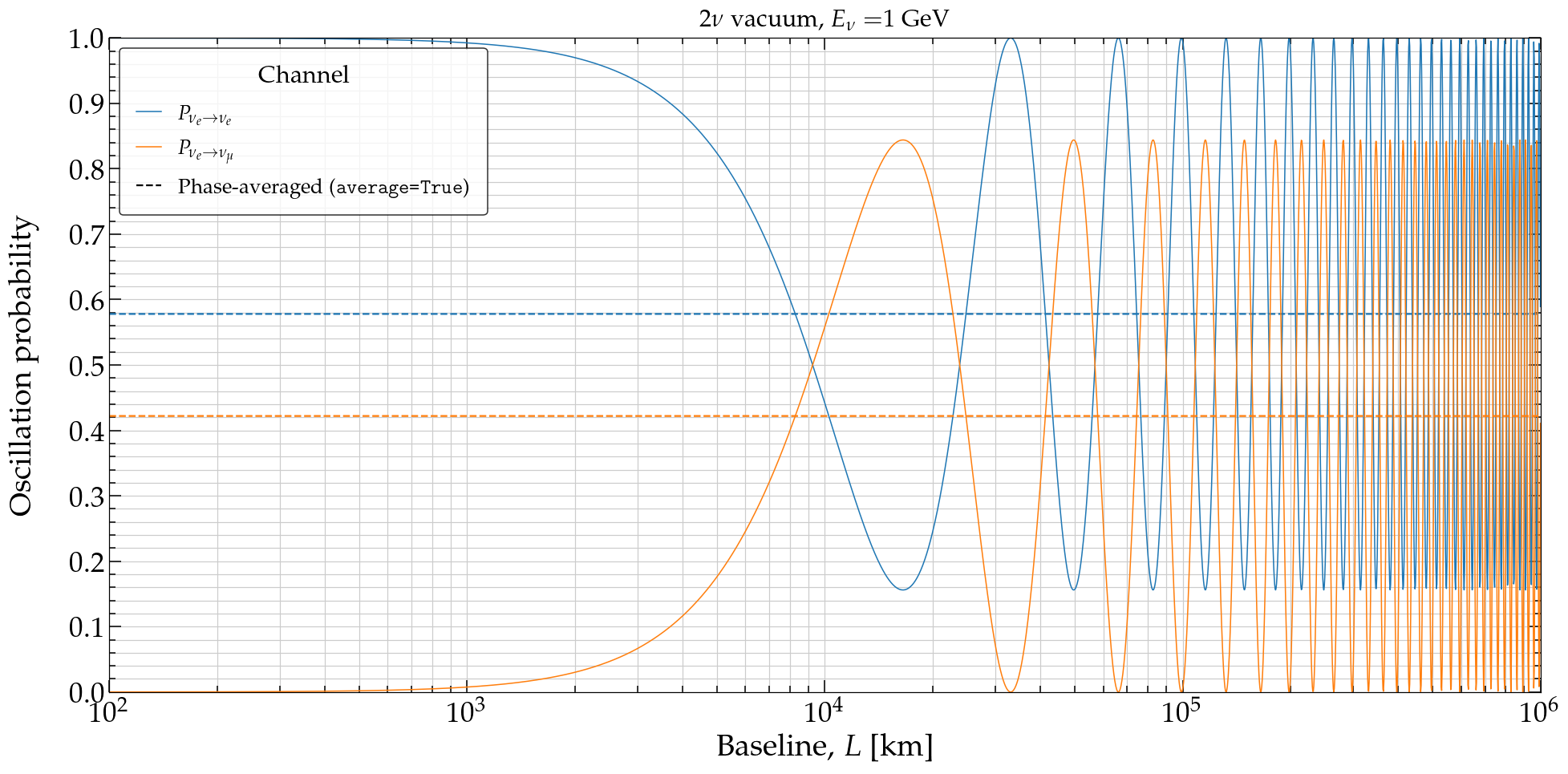 Phase-averaged probabilities — what survives when the oscillation is faster than anything can resolve. notebook 10 |
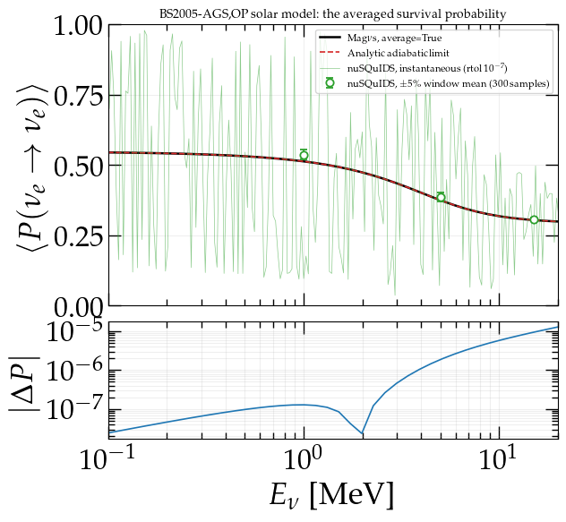 The averaged solar survival probability, returned directly in about 0.7 s. The green trace is the instantaneous probability another code returns, thrashing between 0.15 and 0.9. notebook 25 |
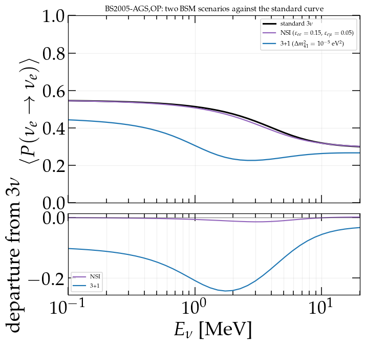 BSM against the standard curve: NSI and a sterile state on a real BS2005 solar model, with the departure below. notebook 13 |
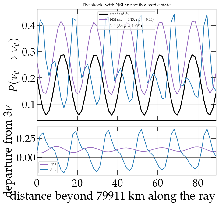 The same two scenarios on a supernova shock, where the identical $\varepsilon$ moves the answer thirty times further. notebook 14 |
Table of Contents
- Installation
- What you can compute
- When is Magnus a win?
- Adiabatic + Magnus hybrid strategy for extreme accumulated phases
- Phase-averaged probabilities for astrophysical neutrinos
- When is Magnus not the right tool?
- Magnus against other oscillation codes
- Two ways to use Magnus
- What Magnus computes
- Available oscillation-probability functions
- Numerical engine
- Performance
- Pre-packaged plotting tools
- Accuracy and validation
- Documentation
- File Tree
- Continuous Integration
- Requirements
- Changelog
- How to Cite
- License
- Author
When is Magnus a win?
Compared to solving the propagation ODE directly (e.g., with an adaptive Runge–Kutta solver), Magnus wins when one or more of these apply:
-
The matter profile varies slowly compared to the oscillation length. A Magnus slab is exact for a constant Hamiltonian no matter how many oscillation cycles it spans, so the slab size is set by how fast the profile changes, not by how fast the phase winds. An ODE solver must resolve every oscillation. For a 1-GeV neutrino crossing the Earth (PREM profile), Magnus needs ~10 slabs plus the ~16 layer crossings, versus thousands of right-hand-side evaluations for
solve_ivp— measured: ~2 ms vs ~360–700 ms per probability at comparable accuracy. -
You scan over energy and/or direction (spectra, oscillograms, sensitivity studies). The Magnus kernel is built from fixed, data-independent matrix operations, so slabs — and, for the standard/NSI/LIV Hamiltonians, the entire energy axis — evaluate as batched NumPy/BLAS calls. Adaptive ODE integration is inherently sequential and cannot share steps across energies. Measured on an idle machine: a 200-energy Earth-crossing scan takes 17 ms with the numba backend and 31 ms without it (0.08 and 0.15 ms per energy); a 100×100 oscillogram takes ~2 s.
-
Unitarity matters more than raw local error — long baselines, small probabilities, CP/T asymmetries. Runge–Kutta iterates drift off the unitary manifold (probability leaks of ~10⁻⁶ at typical tolerances, growing with baseline); the Magnus route has no leakage to leak, ever (rows sum to 1 to ~10⁻¹⁴).
-
You want arbitrary physics with no per-model work: any number of flavors, any Hermitian Hamiltonian — sterile neutrinos, NSI, Lorentz-invariance violation, or your own matrix function of energy and position.
When is it not the best tool? For a single probability at a single energy,
any method is fast enough. For extreme accumulated phases — e.g.,
~10-MeV neutrinos crossing most of the Sun (~10⁴ rad of matter-dominated
phase) — the plain Magnus slab-refinement method can need a very large slab
count, and warns (ToleranceNotAchievedWarning) instead of failing silently
if it hits its caps first. This regime is now handled automatically:
osc_prob_matter_std_potential,
osc_prob_matter_nsi, osc_prob_liv, and every wrapper built on them
(including all osc_prob_*_sun* functions) handle exactly this regime
automatically, via strategy='auto' (the default): see Adiabatic + Magnus
hybrid strategy
below. A tight-tolerance ODE solver remains the best reference for
validation regardless — Magnus's own test suite uses
scipy.integrate.solve_ivp at rtol=1e-12 as ground truth.
Adiabatic + Magnus hybrid strategy for extreme accumulated phases
For a position-dependent Hamiltonian with no user-supplied slab edges, every
matter/NSI/LIV oscillation-probability function accepts a strategy keyword:
'auto' (default), 'hybrid', or 'magnus'.
'magnus'uses only the Magnus-expansion machinery described above — the exact behavior of Magnus as it was before the adiabatic strategy was added.'hybrid'additionally tries an adiabatic-transport-plus-Magnus-patch propagator (magnus.adiabatic.hybrid_propagator): away from an eigenvalue crossing of the instantaneous Hamiltonian, the evolution operator is computed via the instantaneous eigenbasis (a dynamical + geometric phase, cheap regardless of how large the accumulated phase is); near a genuine MSW resonance, a short, exact Magnus patch is stitched in via the exact composition law of quantum evolution. The result is exactly unitary regardless of the approximation's accuracy, and the whole computation is self-certified by tightening every internal tolerance knob until two successive results agree. Works for any number of flavors and any number of simultaneous or sequential resonances — not just the two-flavor case.'auto'tries'hybrid'first, silently falling back to'magnus'for any point where it does not apply or fails to self-certify.
import magnus.oscprob as oscprob
import magnus.globaldefs as gd

# 8 MeV, most of the way through the Sun: deep in the regime that used to
# need a very large slab count under strategy='magnus'.
P = oscprob.osc_prob_3nu_sun(8.0*gd.UNIT_MEV, 0.9*gd.SUN_RADIUS*gd.UNIT_KM, 0.0)
# strategy='auto' by default: warning-free, and matches solve_ivp to ~1e-4.
See the full derivation, validation, and worked examples in the docs.
Phase-averaged probabilities for astrophysical neutrinos
A neutrino from an astrophysical source arrives with an oscillation phase of
order 10¹⁵ — far beyond what the source distance, the production region, or the
detector's energy resolution pin down. Every oscillatory term is averaged away
by the measurement, and the probability collapses to the exact
$L/E \to \infty$ limit,
P(\nu_\alpha \to \nu_\beta) = \sum_i |V_{\alpha i}|^2 |V_{\beta i}|^2
Pass average=True to any oscillation-probability function to get it:
import magnus.oscprob as oscprob
import magnus.globaldefs as gd

osc = gd.load_nufit_params('NuFIT 6.1')
P = oscprob.osc_prob_3nu_vacuum(1.0*gd.UNIT_TEV, 1.0e8*gd.UNIT_KM,
                                average=True, **osc)
This is not an approximation to be refined — it is the exact limit, and it costs one matrix product (~20 μs) instead of resolving 10¹⁵ radians of phase. For vacuum it does not depend on energy or baseline at all, so one matrix serves an entire flux calculation. Matter, NSI and LIV are covered too, and a position-dependent profile decoheres in the eigenbasis at production, is carried along the levels of the instantaneous Hamiltonian — with exact level-crossing probabilities where the evolution stops being adiabatic — and is read out at detection.
Whether the average applies is checked rather than assumed: a pair of eigenvalues whose relative phase is neither ≫ 2π nor ≪ 1 is in no valid limit, and the request warns instead of returning a number the physics does not support. Asking for an averaged probability at a 1000 km beamline does exactly that.
See the full derivation, diagram, and validation in the docs, and notebook 10 for worked examples across 2–5 flavors and a custom Hamiltonian.
When is Magnus not the right tool?
Magnus solves the unitary Schrödinger equation for a Hermitian Hamiltonian: any truncation of the Magnus series lives in the Lie algebra, so the package is architecturally committed to norm-preserving, reversible evolution. That rules out several classes of problems that show up in neutrino phenomenology:
-
Quantum decoherence. Wave-packet separation, quantum-gravity-induced decoherence, or any model where coherence between mass eigenstates is damped over the baseline requires evolving a density matrix under a non-unitary master equation (e.g., Lindblad/GKSL), not a state vector under a Hamiltonian. Magnus has no dissipative term and cannot represent one.
-
Open-system coupling to a bath. Any scenario where the neutrino exchanges energy or phase information with an environment — collisional decoherence, thermal baths, stochastic scattering beyond the mean-field matter potential — needs a reduced density matrix with dissipators, which is again outside a Hermitian-Hamiltonian, pure-state framework.
-
Neutrino decay. Invisible or visible decay into lighter states removes probability from the system, so the evolution is no longer norm-preserving. A Hermitian effective Hamiltonian cannot encode a decay width — that requires an anti-Hermitian term, which breaks the unitarity the whole method relies on.
-
Self-consistent collective oscillations. Dense-environment (e.g., supernova) neutrino self-interactions, where the effective Hamiltonian depends on the (unknown, evolving) neutrino/antineutrino flavor content itself, are a nonlinear, self-consistent problem. Magnus assumes the Hamiltonian is a known function of energy and position supplied by the caller, not a functional of the solution.
If your problem needs any of the above, look instead at packages built around density-matrix/Lindblad evolution (for decoherence or decay) or dedicated collective-oscillation codes (for self-interaction problems).
Magnus against other oscillation codes
The section above compares Magnus against a general-purpose ODE solver. The more useful comparison is against the other oscillation codes, and it has a clear boundary rather than a winner. Notebook 25 runs it in full, with every code timed in one process on one machine and refereed by a method that is neither code's.
Where a closed form exists, use it. NuOscProbExact solves each slab of constant density in closed form, and an exact algebraic solution beats a truncated series — that is arithmetic, not a defect in either code. Constant density, piecewise-constant PREM and standard three-flavor propagation are exactly what closed forms are built for, and on those Magnus does not win: on an Earth chord the closed form is around 20× cheaper per call, and the sharper a density jump is, the more decisively so.
Magnus earns its place on three axes instead.
-
Reach — accuracy past where a slab product stalls. Composing slabs is second order in the slab width, so halving the width buys a factor of four; the Gauss–Legendre Magnus expansion is fourth order and buys sixteen. More importantly the slab product has a floor: on a smooth exponential profile at three flavors its error bottoms out at 2.5 × 10⁻¹¹ near 16 000 slabs and then rises — past that point the round-off of composing so many matrix products costs more than another halving buys, so 32 768 slabs is worse than 16 384. There is no setting below that floor. Magnus continues to 2.9 × 10⁻¹³.
-
Generality — an arbitrary
H(t), and five flavors. A custom Hamiltonian, a BSM term nobody has diagonalized, an interpolated profile read off a simulation: these need no per-model work here, because nothing in the method assumes a form forH. NuOscProbExact has closed forms through four flavors and no five-flavor route at all; at five flavors there is no comparison to draw, which is the same point stated at its limit. -
Pre-packaged observables — the quantity an experiment measures. Over the ray out of the Sun a 5-MeV neutrino accumulates some 13 000 radians of phase, so the instantaneous survival probability at the surface is neither measurable nor stable, and neighboring energies land anywhere between 0.15 and 0.9. What a solar experiment measures is the phase-averaged probability, and
average=Truereturns it directly by transporting along the levels of the instantaneous Hamiltonian instead of propagating. Measured on the same BS2005-AGS,OP model file: Magnus returns 40 averaged energies in about 0.7 s; nuSQuIDS needs about ten minutes merely to reach the solver tolerance at which its output is a probability at all — below it the survival probability reaches 2.83, and a unitarity check passes anyway — and then a further factor of N to average the phase away. Neither NuOscProbExact nor nuSQuIDS offers an averaging flag — this is a different algorithm for the question actually being asked, not the same algorithm run faster.
The short version: piecewise-constant and standard, use a closed form; smooth, exotic, five-flavor, or phase-averaged, use this. The full comparison — a case-by-case table of which to reach for, and the measurements behind each row — is on the Against other codes documentation page.
Two ways to use Magnus
Magnus works both as an importable Python module (the full API —
arbitrary Hamiltonians, energy/direction scans, NSI, LIV, steriles) and as a
command-line calculator (magnus prob ... — one probability, no Python
required). Use the module for anything programmatic (scans, plots, fitting);
use the CLI for a quick one-off number, a shell script, or to sanity-check a
parameter choice.
As a Python module
import numpy as np
import magnus.oscprob as oscprob
import magnus.globaldefs as gd

# --- Three-flavor vacuum probability at 1 GeV over 1000 km ---
energy = 1.0*gd.UNIT_GEV      # [eV]
L = 1000.0*gd.UNIT_KM         # [eV^-1]
P = oscprob.osc_prob_3nu_vacuum(energy, L)   # 3x3 matrix, P[i][j] = P(nu_i -> nu_j)

# --- Energy scan through the Earth (PREM), nu_e -> nu_mu ---
energies = np.logspace(-0.3, 1.3, 200)*gd.UNIT_GEV
# integration_method defaults to 'gl' (Gauss-Legendre): fastest and most accurate
P_scan = oscprob.osc_prob_3nu_earth(
    energies, costhz=-0.8, L=2.0*6371.0*0.8*gd.UNIT_KM,
    nu_i=gd.NUE, nu_f=gd.NUMU)

# --- Your own Hamiltonian through the Earth ---
# H(energy, l, VCC): VCC is the PREM charged-current potential at position l
import magnus.hamiltonians as hamiltonians
osc = gd.load_nufit_params('NuFIT 6.1', 'NO')
h_vac = np.asarray(hamiltonians.hamiltonian_3nu_vacuum_energy_independent(
    osc['s12'], osc['s23'], osc['s13'], osc['dCP'], osc['D21'], osc['D31']))

def H(energy, l, VCC):
    return (1.0/energy)*h_vac + np.asarray(VCC)[..., None, None]*np.diag([1.0, 0.0, 0.0])

P = oscprob.osc_prob_earth(H, energy, loc_ini='fermilab', loc_fin='homestake')

# --- Fully generic: any Hamiltonian function of position ---
P = oscprob.osc_prob(lambda l: h_vac/energy, t_ini=0.0, t_fin=L)  # H(l) -> (d, d)
Oscillation parameters default to the NuFit 6.1 best fit (normal ordering);
pass s12, D31, dCP, ..., or nubar=True, to change them. Find many
worked examples — vacuum, matter, Earth, Sun, oscillograms, biprobability
plots, steriles, NSI, LIV — in the Jupyter notebooks.
Mixing angles are sines by default, which is what load_nufit_params returns.
angles takes any of the four conventions a fit might be published in, so a
parameter set can be typed in as printed rather than converted by hand:
# sin^2, the form global fits report
P = oscprob.osc_prob_3nu_vacuum(energy, L, s12=0.308, s23=0.470, s13=2.215e-2,
                                dCP=3.70, D21=7.49e-5, D31=2.513e-3, angles='sin2')

# or degrees, straight off the NuFit table -- dCP included
P = oscprob.osc_prob_3nu_vacuum(energy, L, s12=33.76, s23=43.28, s13=8.62,
                                dCP=212.0, D21=7.49e-5, D31=2.513e-3, angles='deg')
'sin' (default), 'sin2', 'rad' and 'deg'; under 'deg' the CP phases are
read as degrees too. Every function that takes a mixing angle takes it, the
magnus prob command line included, and load_nufit_params(angles=...) returns a
set in the matching convention — pass the same value to both, since sines read
as degrees are about fifty times too small and would otherwise give a converged,
unitary, wrong answer. That particular pairing raises a
MixingAngleConventionWarning.
As a command-line calculator
Installing the package also installs a magnus command
(equivalently, python -m magnus), for computing a single probability
without writing any Python. magnus prob --help lists every flag; the
full CLI reference documents
all of them. A few real examples (verified output, this version):
$ magnus prob --flavors 3 --environment vacuum \
    --energy 1 --energy-unit GeV --baseline 1300 --baseline-unit km
Magnus 1.0.0rc1 -- osc_prob_3nu_vacuum
E = 1 GeV, L = 1300 km

            nu_e   nu_mu  nu_tau
nu_e      0.9297  0.0085  0.0618
nu_mu     0.0311  0.3885  0.5804
nu_tau    0.0393  0.6029  0.3578
$ magnus prob --flavors 3 --environment earth \
    --energy 1 --energy-unit GeV --costhz -0.8 --baseline 10193.6 --baseline-unit km
Magnus 1.0.0rc1 -- osc_prob_3nu_earth
E = 1 GeV, L = 10193.6 km

            nu_e   nu_mu  nu_tau
nu_e      0.9128  0.0863  0.0009
nu_mu     0.0629  0.6681  0.2690
nu_tau    0.0243  0.2456  0.7301
A single channel (rather than the full matrix), and NSI/LIV/sterile flags, work the same way:
$ magnus prob --flavors 3 --environment vacuum --energy 1 --energy-unit GeV \
    --baseline 1300 --baseline-unit km --nu-i e --nu-f mu
Magnus 1.0.0rc1 -- osc_prob_3nu_vacuum
E = 1 GeV, L = 1300 km

P = 0.0085

$ magnus prob --flavors 3 --environment matter --scenario nsi --rho 2.7 \
    --eps-ee 0.06 --eps-em -0.06 \
    --energy 1 --energy-unit GeV --baseline 1000 --baseline-unit km
Magnus 1.0.0rc1 -- osc_prob_3nu_matter_nsi_constant_density
E = 1 GeV, L = 1000 km

            nu_e   nu_mu  nu_tau
nu_e      0.9898  0.0093  0.0009
nu_mu     0.0093  0.9906  0.0001
nu_tau    0.0009  0.0001  0.9990
Pass --json for machine-readable output (e.g., to pipe into jq or another
script) instead of the table.
What Magnus computes
- Flavors: 2ν, 3ν, 4ν (3+1), 5ν (3+2) via dedicated wrappers; any number
of flavors via the generic
osc_prob. - Environments: vacuum, constant-density matter, exponentially falling density, the Earth (PREM, including chords between named detector sites), the Sun; or any density profile you supply.
- Beyond the Standard Model: non-standard interactions (NSI),
CPT-odd Lorentz-invariance violation (LIV), and — via
osc_prob,osc_prob_earth,osc_prob_sun— arbitrary user Hamiltonians. - Neutrinos and antineutrinos, single energies or arrays, full probability matrices or single channels.
Available oscillation-probability functions
Every combination of environment and scenario below has a dedicated,
explicitly-named osc_prob_{N}nu_... function for N in {2, 3, 4, 5}
(e.g. osc_prob_3nu_matter_nsi_constant_density) — see
the full listing with signatures
in the docs. For anything not covered here — any other number of flavors,
or a Hamiltonian this table doesn't anticipate — use the generic
osc_prob/osc_prob_earth/osc_prob_sun entry points directly (see
Quick start above).
| Environment | Scenario | Function pattern ({N} = 2, 3, 4, 5) |
|---|---|---|
| Vacuum | Standard | osc_prob_{N}nu_vacuum |
| Vacuum | LIV | osc_prob_{N}nu_vacuum_liv |
| Matter, constant density | Standard | osc_prob_{N}nu_matter_constant_density |
| Matter, constant density | NSI | osc_prob_{N}nu_matter_nsi_constant_density |
| Matter, constant density | LIV | osc_prob_{N}nu_matter_liv_constant_density |
| Matter, exponential density | Standard | osc_prob_{N}nu_matter_exp_density |
| Matter, exponential density | NSI | osc_prob_{N}nu_matter_nsi_exp_density |
| Matter, exponential density | LIV | osc_prob_{N}nu_matter_liv_exp_density |
| Earth (PREM) | Standard | osc_prob_{N}nu_earth |
| Earth (PREM) | NSI | osc_prob_{N}nu_earth_nsi |
| Earth (PREM) | LIV | osc_prob_{N}nu_earth_liv |
| Sun | Standard | osc_prob_{N}nu_sun |
| Sun | NSI | osc_prob_{N}nu_sun_nsi |
| Sun | LIV | osc_prob_{N}nu_sun_liv |
The command-line calculator exposes this
same table via --environment/--scenario/--flavors.
Numerical engine
- Magnus expansion to order 6, with the term recursion verified term-by-term against Blanes, Casas, Oteo & Ros, Phys. Rep. 470, 151 (2009).
- Three integration methods. The default,
'gl'— Gauss–Legendre commutator-free integrators of orders 2/4/6 that need only 1/2/3 Hamiltonian evaluations per slab (Blanes, Casas & Ros, BIT 40, 434 (2000)) — is both the fastest and the most accurate for a smooth-per-slab profile, which layer-aligned slabs make the common case.'trapezoid'and'simpson'(cumulative quadrature overn_tpts_per_slabpoints) remain available, and are the safer choice if the Hamiltonian has a kink or a discontinuity inside a slab. - Exactly unitary exponentials from the eigendecomposition of the (anti-Hermitian) Magnus operator, batched over slabs and energies.
- Magnus expansion terms at any order:
magnus.expansiontermsderives them from the Bernoulli recursion symbolically, in exact rational arithmetic, which is what verifies the hard-coded coefficients rather than taking them on trust. Orders 1–6 are written out inline, 7–10 generated. - Method-aware refinement caps:
max_n_slabsdefaults to the cap that suits the integration method (20000 for'gl', 2000 for the quadrature methods), since'gl'costs 1–3 Hamiltonian evaluations per slab against the others'n_tpts_per_slab. A shared cap made'gl'report non-convergence on problems it had in fact resolved more accurately than the quadrature methods managed within the same cap. - Adaptive refinement until two successive levels agree within
rtol/atol, with a phase-based starting slab count, warm starts across scan points, and an always-on warning if the refinement caps are hit before convergence. Note that is an agreement, not a bound on the error — the ladder never estimates the accuracy of what it returns. See whatrtol/atolactually control. - Slab edges aligned with the PREM layer boundaries, so the high-order quadrature never integrates across a density discontinuity.
- Silent vectorization: Hamiltonian and density-profile functions that accept position arrays are detected and used automatically (with a safe scalar fallback); profile evaluations are cached across repeated grids; for standard/NSI/LIV scans, the whole energy axis is batched through the kernel.
Performance
Measured on a laptop, 3ν through the Earth (PREM), default tolerance 10⁻³:
| Workload | Time |
|---|---|
| Single probability (1 GeV, cos θz = −0.8) | ~2 ms |
| 200-energy scan, one direction | 76 ms (0.4 ms/energy) |
| 100 × 100 oscillogram (energy × direction) | ~2 s |
Reference: solve_ivp DOP853, single probability, rtol 10⁻⁶ |
~360 ms |
Write your H_func so it accepts an array of positions
Those figures assume the fast path. If you pass your own Hamiltonian to
osc_prob, the single largest factor under your control is whether it can be
evaluated for many positions at once.
The engine samples the Hamiltonian at every quadrature node of every slab —
often a few hundred positions for one probability, repeated at each level of
the adaptive refinement. It therefore tries a single vectorized call,
H_func(array_of_positions), and uses the result if it has the right shape and
agrees with a scalar spot-check. If that fails it falls back to a Python loop,
one call per position: correct, but measured 4.6× slower on a 3ν
exponential-density profile (7.8 ms → 1.7 ms per osc_prob call), with
bit-identical output.
# Slow: one position at a time
def H_func(l):
    VCC = matter.VCC_func(l, num_density_e_func)
    return (1.0/energy)*h_vac + hamiltonians.hamiltonian_3nu_matter(VCC)

# Fast: the same physics, all positions at once
e00 = np.diag([1.0, 0.0, 0.0])
def H_func(l):
    l = np.asarray(l, dtype=float)
    VCC = VCC_central*np.exp(-(l/gd.UNIT_KM)/l_scale)   # an array
    return (1.0/energy)*h_vac + VCC[..., None, None]*e00
The [..., None, None] is the whole trick: it turns one potential per position
into a stack of matrices, so NumPy broadcasts instead of Python looping. Note
that this is a property of your function, not of osc_prob — the engine's own
inner loops are already vectorized.
Two things worth knowing:
- A Hamiltonian that ignores its argument (constant density) is detected separately and broadcast, so it is already fast and needs no change.
- Since 1.0.0 the fallback raises
magnus.magnus.ScalarHamiltonianWarningonce per session, naming the fix. Before that it was silent, which is why the slow path is easy to sit on indefinitely — the shipped example notebooks all did.
Pre-packaged plotting tools
Magnus ships the figures its own notebooks use, so a plot is one call rather than thirty lines of Matplotlib. Matplotlib is a dependency, so there is nothing extra to install.
import numpy as np
import magnus.globaldefs as gd
import magnus.oscprob as oscprob
from magnus import plotting

energies = np.linspace(0.5, 10.0, 120)*gd.UNIT_GEV
P = np.asarray(oscprob.osc_prob_3nu_vacuum(
    energies, np.full(120, 1300.0*gd.UNIT_KM)))

fig, ax = plotting.plot_probability_vs_energy(
    energies/gd.UNIT_GEV,
    [{'y': P[:, 1, 0], 'label': plotting.prob_label(1, 0)}],
    nu_i=1, nu_f=0)
prob_label(1, 0) returns $P_{\nu_\mu \to \nu_e}$, so channel labels are
consistent without being retyped.
| Function | Shape it draws |
|---|---|
plot_curves |
curves against any swept variable, with an optional relative-error subpanel |
plot_probability_vs_energy, ..._vs_baseline |
presets over it, with labels, scales and tick spacings fixed |
plot_curves_stacked |
small multiples -- one panel per configuration down a shared abscissa |
plot_probability_with_profile |
a probability above the matter profile that produced it |
plot_probability_with_average |
instantaneous against phase-averaged |
plot_biprobability |
the CP ellipse, neutrino against antineutrino |
plot_oscillogram |
the two-dimensional map across zenith angle and energy |
The point is consistency rather than brevity: the panels of a stacked figure
must share limits, scales and tick spacings or the reader's comparison between
them is meaningless, and that is what drifts when each figure is built by hand.
House defaults live in HOUSE_FIGSIZE, HOUSE_LEGEND_KW and friends; every
function returns the fig/ax, so anything can still be overridden.
Full documentation: Pre-Packaged Plotting Tools.
Accuracy and validation
The test suite (running in CI on Python 3.10–3.13) validates:
- Magnus terms against an independently coded Bernoulli-number recursion (orders 1–6, machine precision) and Gauss–Legendre convergence rates (measured error ratios 4/16/64 under slab halving);
- probabilities against closed-form expressions (2ν/3ν vacuum, 2ν
constant-density matter, for neutrinos and antineutrinos) and against
high-accuracy
solve_ivpintegrations (asymmetric profiles with complex Hamiltonians, full PREM Earth crossings); - unitarity, slab-ordering, channel conventions, vectorized-vs-scalar consistency, and the energy-batched scan against the per-point path.
Requested tolerances are targets for the difference between successive refinements — the standard adaptive heuristic — not strict global error bounds; in practice the default 10⁻³ setting delivers ~5 × 10⁻⁴ on Earth crossings (verified against 10⁻⁷-tolerance references).
Documentation
The full documentation is at mbustama.github.io/Magnus. What this page deliberately leaves to it:
| Mathematical method | The Magnus expansion derived term by term: why truncation is exactly unitary at any order, convergence, the position-ordered product, and the two integration methods |
| Expansion terms | The explicit $\Omega_1$, $\Omega_2$, $\Omega_3$ integrals |
| Architecture | How the modules fit together, and which layer to call |
| Engines and dispatch | Which engine answers a call, and how the choice is made |
| Performance | Where the time goes, including the palindromic-chord optimization for Earth trajectories |
| Accuracy and diagnostics | What rtol really controls, what each safeguard cannot catch, and every warning explained |
| Against other codes | The full cross-code comparison against NuOscProbExact and nuSQuIDS: which to reach for, case by case, and the measurements behind it |
| Numerical recipes | Runnable snippets for the common tasks |
| Tutorials | All 27 notebooks, with what each one is for |
| API reference | Every public function, generated from the source |
File Tree
The top level only; the complete
listing, with a comment
on every file, is in the documentation. Both are generated from git ls-files,
so neither can drift from the repository:
Magnus/
├── .github/                        # GitHub Actions workflows: tests, lint, notebooks, docs, publishing
├── .gitignore                      # Build, cache and generated-output artifacts
├── CHANGELOG.md                    # Version history (Keep a Changelog format)
├── CITATION.cff                    # Machine-readable citation metadata; drives GitHub's "Cite this repository"
├── LICENSE                         # GNU GPL v3 (GPL-3.0-only), the full license text
├── README.md                       # This file
├── docs/                           # Sphinx documentation configuration and source
├── fig/                            # Plots produced by the example notebooks
├── img/                            # Figures used by the documentation
├── notebooks/                      # Numbered Jupyter notebooks -- see docs/source/tutorials.rst
├── pyproject.toml                  # Build system, dependencies, and the `magnus` console-script entry point
├── tools/                          # Standalone utilities that are not part of the package
├── src/                            # The package itself -- the only thing a `pip install` delivers
└── tests/                          # Test suite (pytest; runs in CI)
Continuous Integration
Every push runs the full suite on Python 3.10-3.13, executes all 27
notebooks, builds the documentation with warnings-as-errors, and lints with
Ruff — the badges at the top of this page report those runs. The workflows
live in .github/workflows/.
Requirements
numpy, scipy (>= 1.9), joblib — see
src/requirements.txt.
matplotlib is among them too, so
magnus.plotting -- the pre-packaged plotting tools --
works in any installation with nothing further to install.
Run the tests with:
pip install -e '.[test]' && pytest tests/
(tests/conftest.py puts src/ on the path, so pip install -r src/requirements.txt pytest works too; installing the package is what CI does,
and it additionally exercises the magnus console script.)
The test extra also pulls in pytest-cov, so the same suite can report what
it covers:
pytest tests/ --cov --cov-report=term-missing
Branch coverage, the measured source tree and the omitted files are configured
in [tool.coverage.run] in pyproject.toml, so a bare --cov measures the
same thing locally and in CI. Branch coverage is on deliberately: line coverage
alone flatters this package, because oscprob.py is mostly thin wrappers that a
single parametrized test sweeps in one pass, and the interesting question is
whether the dispatch chain, the refinement caps and the warning paths are each
taken in both directions. Expect the suite to run measurably slower under
instrumentation.
The documentation's code examples are executed for real at build time, so a broken one fails CI — but only in the full Sphinx build, which takes minutes. To check them directly, in about a second per page:
python3 docs/check_doc_snippets.py --rst-only
It runs every .. jupyter-execute:: block, in the RST pages and in the
docstrings autoapi renders. Drop --rst-only to include the docstrings, which
is thorough but as slow as the examples themselves. This exists because the
fast documentation build stubs those blocks out: it validates the prose and the
cross-references while saying nothing about the code, so a page can build
cleanly and still be broken.
Changelog
See CHANGELOG.md (also rendered in the docs) for a version-by-version history of what changed and why.
How to Cite
If you use Magnus in your academic work or scientific publications, please cite it and link to the source repository:
Mauricio Bustamante (2026). Magnus: neutrino oscillation probabilities via the Magnus expansion. GitHub Repository: https://github.com/mbustama/Magnus.
Methodology References:
- Sergio Blanes, Fernando Casas, José A. Oteo & José Ros (2009). The Magnus expansion and some of its applications. Physics Reports, 470(5-6), 151-238. doi:10.1016/j.physrep.2008.11.001.
- Sergio Blanes, Fernando Casas & Javier Ros (2000). Improved high order integrators based on the Magnus expansion. BIT Numerical Mathematics, 40(3), 434-450. doi:10.1023/A:1022311628317.
- Adam M. Dziewonski & Don L. Anderson (1981). Preliminary reference Earth model. Physics of the Earth and Planetary Interiors, 25(4), 297-356. doi:10.1016/0031-9201(81)90046-7.
License
Magnus is released under the GNU General Public License v3.0 only
(GPL-3.0-only). The full text is in LICENSE.
In short: you are free to use, study, modify, and redistribute it, including for commercial purposes, provided that derivative works are distributed under the same license and with source available. If you are unsure whether your intended use is compatible, read the license itself rather than this summary.
Author
Mauricio Bustamante (mbustamante@gmail.com)
1 maintainer

Release files for magnuspy 1.0.0
For a detailed explanation of source distributions (sdists) and built distributions (wheels), please see the package formats documentation.
Source distribution (sdist)
| File | Size | Uploaded | |
|---|---|---|---|
| magnuspy-1.0.0.tar.gz | 524.4 kB | Details |
Built distribution (wheel)
| File | Interpreter | ABI | Platform | Reset |
|---|---|---|---|---|
| magnuspy-1.0.0-py3-none-any.whl | Python 3 | none | any | Details |
Total release size: 874.0 kB
Release files / magnuspy-1.0.0.tar.gz
| Download URL | magnuspy-1.0.0.tar.gz |
|---|---|
| Size | 524.4 kB |
| Tags | Source |
|
SHA-256 checksum How to use checksums |
2dbf0fd280f15ee23aec38cd609298e8d99c38c7710f15f8a6675bfa43e27887
|
|
BLAKE2b-256 checksum How to use checksums |
51b4c376d6aa20537e3b6e271462d416cc05881a4675ba3c523d5f70725eff71
|
| Upload date | |
|
Uploaded using Trusted Publishing? What is trusted publishing? |
Yes |
| Uploaded via |
twine/7.0.0 CPython/3.13.14
|
Provenance
Provenance describes where a file came from. On PyPI, provenance is shared via attestations, which provide a verifiable record of the build or publishing details. View details, limitations and caveats.


PyPI Publish Attestation
PyPI verified that this artifact, at this checksum, originated from the publisher listed below.
Signed by GitHub Actions, verified by PyPI on Aug 13, 2026.
Transparency logRelease files / magnuspy-1.0.0-py3-none-any.whl
| Download URL | magnuspy-1.0.0-py3-none-any.whl |
|---|---|
| Size | 349.6 kB |
| Tags | Python 3 |
|
SHA-256 checksum How to use checksums |
9ec42a308b47abd61a4a00ee7d82447615bcf00d63ebe369965bd99b83a23cb4
|
|
BLAKE2b-256 checksum How to use checksums |
b808c273a707783a3ed2940b39db23a097fcb3df7e04bb5c958537831eec061d
|
| Upload date | |
|
Uploaded using Trusted Publishing? What is trusted publishing? |
Yes |
| Uploaded via |
twine/7.0.0 CPython/3.13.14
|
Provenance
Provenance describes where a file came from. On PyPI, provenance is shared via attestations, which provide a verifiable record of the build or publishing details. View details, limitations and caveats.
PyPI Publish Attestation
PyPI verified that this artifact, at this checksum, originated from the publisher listed below.
Signed by GitHub Actions, verified by PyPI on Aug 13, 2026.
Transparency log












