
MantiShrimp


MantiShrimp is a Python package for agent-based modelling of killer immune cell–tumour cell interactions and Bayesian analysis of the resulting cell-level event counts.
The package has two connected layers:
- an off-lattice, two-dimensional ABM using the refined Hookean interaction rules from Szonja Skenderovic's thesis;
- the four Bayesian count models from the Orca inference work, applicable to either contacts per killer cell or kills per killer cell.
The historical scripts and notebooks remain in the repository as provenance.
New work should use the importable package under src/mantishrimp.
ABM demonstration
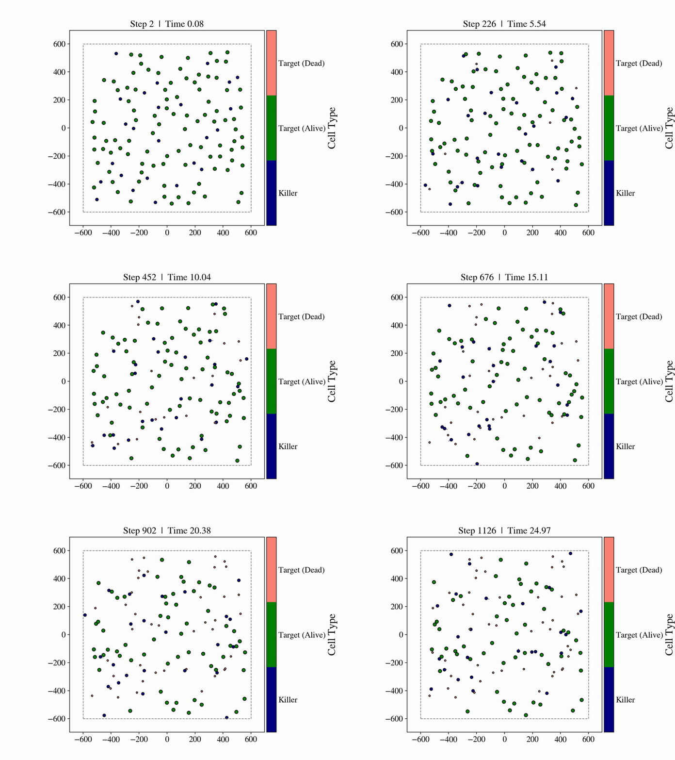
Blue agents are killer immune cells, green agents are living tumour targets, and salmon agents are dead targets. Cells move continuously in the off-lattice domain; killer-target proximity can lead to stochastic synapse formation, damage accumulation, and target death. The animation is a visual illustration of one run rather than a calibrated biological prediction. A full-resolution version is also available.
Install
python -m pip install mantishrimp
python -m pip install 'mantishrimp[inference]'
python -m pip install 'mantishrimp[all]'  # inference and plotting
Python 3.10 or newer is supported.
Simulate killer–target interactions
from mantishrimp import SimulationConfig, simulate

config = SimulationConfig.szonja_baseline(
    n_killers=25,
    n_targets=100,
    duration=25.0,  # shortened from the 80-minute thesis baseline
    seed=42,
)
result = simulate(config)

print(result.summary())
print(result.contacts_per_cell())
print(result.kills_per_cell())
SimulationResult contains:
snapshots: one row per recorded cell and time point;events: contact, synapse, and death events with killer/target identities;final_cells: the final recorded population state;config: the complete typed simulation configuration.
Contacts and synapses are deliberately different. A contact is a proximity episode; a synapse is a stochastic bound state formed during contact. This keeps the biological mechanism separate from the observable used for inference.
Infer heterogeneity from ABM results
The inference layer asks a population-level question: are killer cells consistent with one common event rate, or is there evidence for inactive cells, continuous rate heterogeneity, or both? It operates on one integer count per killer cell. That count can be either the number of contact episodes or the number of attributed kills.
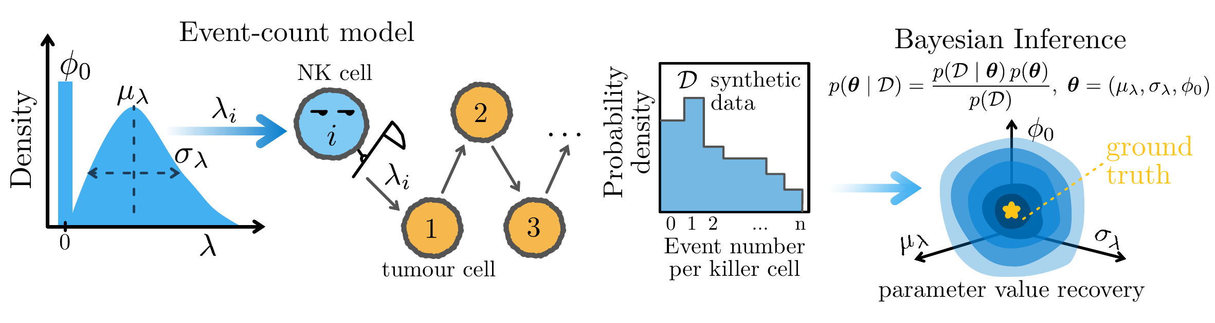
The workflow above has three steps:
- Each killer cell
ihas a latent event rateλᵢ. - Over exposure time
Tᵢ, its observed count is modelled asNᵢ | λᵢ, Tᵢ ~ Poisson(λᵢTᵢ). - Bayesian inference combines the count likelihood with the parameter priors
to estimate
p(θ | D), whereθ = (μλ, σλ, φ₀).
Here μλ is the mean event rate among active killer cells, σλ is their
between-cell rate variation, and φ₀ is the
fraction of structurally inactive killer cells. Zero-count cells are retained:
an observed zero can arise either from an active Poisson process that happened
to produce no events or, in zero-inflated models, from the inactive component.
The default exposure is the simulated duration, although aligned per-cell
exposures can be supplied directly.
Four candidate population models
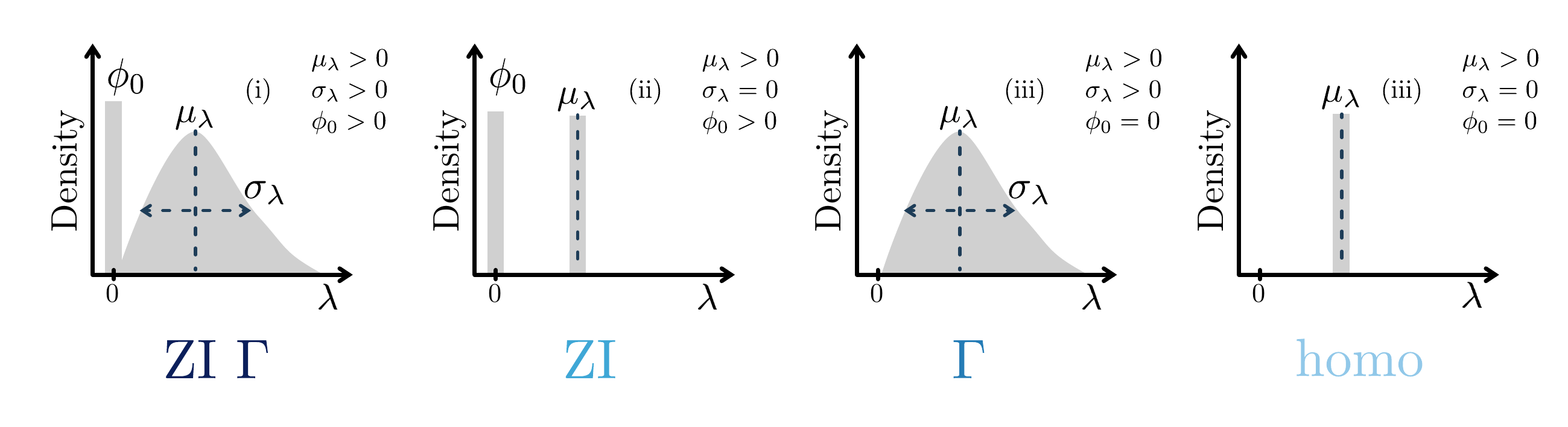
The figure expresses the four models as restrictions of the same latent-rate
distribution. The grey/blue mass at zero is φ₀; the positive-rate
distribution has mean μλ and standard deviation σλ.
| Package name | Figure | Parameter restriction | Count distribution | Interpretation |
|---|---|---|---|---|
homo |
homo | σλ = 0; φ₀ = 0 |
Poisson | one shared rate |
Z2P |
ZI | σλ = 0; φ₀ > 0 |
zero-inflated Poisson | shared active rate plus inactive cells |
Dis2P |
Γ | σλ > 0; φ₀ = 0 |
negative binomial | Gamma-distributed active-cell rates |
hetero3 |
ZI Γ | σλ > 0; φ₀ > 0 |
zero-inflated negative binomial | Gamma rates plus inactive cells |
For the Gamma models, integrating the cell-specific λᵢ values out of
the Poisson likelihood gives the negative-binomial count distribution. This
lets the model estimate continuous cell-to-cell variation without sampling a
separate rate for every killer.
The original vector figures are available as the inference workflow PDF and the four-model PDF.
Fit contacts and kills separately
Install the inference extra, then fit the same candidate suite to each
observable:
from mantishrimp.inference import evidence_table, infer_contacts, infer_kills

contact_fits = infer_contacts(
    result,
    draws=1000,
    chains=2,
    random_seed=42,
)
kill_fits = infer_kills(
    result,
    draws=1000,
    chains=2,
    random_seed=43,
)

print(evidence_table(contact_fits))
print(evidence_table(kill_fits))
Contacts and kills should be analysed as separate datasets because they answer different biological questions: contact inference characterises encounter opportunity, whereas kill inference combines encounter, synapse, damage, and cytotoxic competence.
Posterior recovery and model comparison
Models are fitted with PyMC Sequential Monte Carlo (SMC). Each FitResult
contains posterior samples for parameter recovery and a log marginal
likelihood for model comparison. With equal prior model probabilities,
BF(A, B) = p(D | M_A) / p(D | M_B) = exp(log Z_A - log Z_B)
The posterior answers which parameter values are plausible within a model;
the Bayes factor answers which population model is better supported by the
observed counts. evidence_table, bayes_factor_matrix, and the plotting
helpers expose both views. Raw count arrays can also be fitted with
fit_count_model or fit_model_suite.
This count likelihood is an observation model for ABM outputs; it does not by itself infer Hookean force constants, motility parameters, or causal cell-cell network structure. Those would require a separate calibration or simulation-based inference layer.
Package map
config.py: validated simulation parameters and the Szonja baseline;simulation.py: Hookean ABM engine;results.py: event-count extraction and result persistence;inference.py: Orca-derived Bayesian model suite;validation.py: synthetic Poisson/Gamma/zero-inflated generators;analysis.py: evidence, posterior, sweep, and persistence helpers;plotting.py: reusable posterior and Bayes-factor plots.
See the scientific model contract and notebook-function migration map.
Authors and citation
MantiShrimp was developed by Elephes Sung, Szonja Skenderovic, Yixuan Li, and
Ruben Perez-Carrasco at the Department of Life Sciences, Imperial College
London. Elephes Sung and Szonja Skenderovic contributed equally. See
AUTHORS.md for
author details and
CITATION.cff
for machine-readable citation metadata.
Development
python -m pip install -e '.[all,test]'
pytest
The package is currently alpha software. Before using it for biological claims, calibrate the time/space units, parameter priors, and observation process against the experiment being modelled.
1 maintainer

Metadata
1 maintainer
Release files for mantishrimp 0.3.0
For a detailed explanation of source distributions (sdists) and built distributions (wheels), please see the package formats documentation.
Source distribution (sdist)
| File | Size | Uploaded | Provenance | |
|---|---|---|---|---|
| mantishrimp-0.3.0.tar.gz | 42.5 kB | With provenance | Details |
Built distribution (wheel)
| File | Interpreter | ABI | Platform | Reset |
|---|---|---|---|---|
| mantishrimp-0.3.0-py3-none-any.whl | Python 3 | none | any | Details |
Total release size: 73.2 kB
Release files / mantishrimp-0.3.0.tar.gz
| Download URL | mantishrimp-0.3.0.tar.gz |
|---|---|
| Size | 42.5 kB |
| Tags | Source |
|
SHA-256 checksum How to use checksums |
ffc313bbb81b2542f91d661e8ba9530feecf03c2cf15b1166d952430606be65c
|
|
BLAKE2b-256 checksum How to use checksums |
5224289fb5b0390e7531f2a369612cd5414d3f6733d9445a6e8f69dacda08140
|
| Upload date | |
|
Uploaded using Trusted Publishing? What is trusted publishing? |
Yes |
| Uploaded via |
twine/7.0.0 CPython/3.13.14
|
Provenance
Provenance describes where a file came from. On PyPI, provenance is shared via attestations, which provide a verifiable record of the build or publishing details. View details, limitations and caveats.


PyPI Publish Attestation
PyPI verified that this artifact, at this checksum, originated from the publisher listed below.
Signed by GitHub Actions, verified by PyPI on Oct 14, 2026.
Transparency logRelease files / mantishrimp-0.3.0-py3-none-any.whl
| Download URL | mantishrimp-0.3.0-py3-none-any.whl |
|---|---|
| Size | 30.7 kB |
| Tags | Python 3 |
|
SHA-256 checksum How to use checksums |
5b065dbc44162356acf6984f14678d963c68ba679a95e45c49d1d4f5abec117e
|
|
BLAKE2b-256 checksum How to use checksums |
21ccda52f13fb38d06cf87ac4c3070db80aaa404b41e00c3ff9304ff6e78212a
|
| Upload date | |
|
Uploaded using Trusted Publishing? What is trusted publishing? |
Yes |
| Uploaded via |
twine/7.0.0 CPython/3.13.14
|
Provenance
Provenance describes where a file came from. On PyPI, provenance is shared via attestations, which provide a verifiable record of the build or publishing details. View details, limitations and caveats.
PyPI Publish Attestation
PyPI verified that this artifact, at this checksum, originated from the publisher listed below.
Signed by GitHub Actions, verified by PyPI on Oct 14, 2026.
Transparency logSecurity for mantishrimp 0.3.0
Provenance
Provenance describes where a file came from. On PyPI, provenance is shared via attestations, which provide a verifiable record of the build or publishing details. View details, limitations and caveats.
Full provenance
All 2 files in this release have been uploaded with provenance metadata.
Attestation for mantishrimp-0.3.0.tar.gz
PyPI Publish Attestation
PyPI verified that this artifact, at this checksum, originated from the publisher listed below.
Signed by GitHub Actions, verified by PyPI on Oct 14, 2026.
Transparency logA note on package security
PyPI is a repository for distributing packages, not a service for auditing them. While third-party security researchers and our staff do their best to detect and remove malicious packages, PyPI cannot guarantee the quality, security or suitability of any given package.















