
mantissa-cnn



Classic CNNs, with a C engine.
A small convolutional-network classifier (fit / predict / score) whose
compute runs in mantissa — a
fast, memory-lean neural-network core in C. The Python layer is thin on
purpose: convolution (im2col + GEMM), pooling, the dense head, the fused
softmax-cross-entropy loss and the SGD update all execute in C on zero-copy
float32 buffers. A pure-numpy backend with the identical call signatures
(backend="numpy") serves as the correctness oracle in the test suite and
as a fallback when the engine is absent.
Deliberately minimal: NCHW float32 images, integer class labels, softmax cross-entropy, plain SGD. No autograd graph, no optimizer zoo, no data augmentation. Layers allocate their forward/backward scratch once per batch shape and reuse it across batches and epochs — steady-state training does no per-batch allocation.
Install
pip install mantissa-cnn
Requires the engine mantissa-core >= 0.2.1 (the release that adds the CNN
primitives). From a checkout (works today, no PyPI needed): clone this repo
next to mantissa, build the
engine (make dist there), then pip install -e . here — the package finds
the sibling checkout automatically.
Quickstart
# datasets never download implicitly — fetch explicitly, once:
python -m mantissa_cnn.datasets download mnist     # or: download all
python -m mantissa_cnn.datasets list
from mantissa_cnn import models, datasets

X_train, y_train, X_test, y_test = datasets.load("mnist")
net = models.lenet5()                    # C engine; backend="numpy" also works
print(net.summary())
net.fit(X_train, y_train, epochs=3, batch_size=32, lr=0.01, verbose=True)
print(net.score(X_test, y_test))
Or compose your own:
from mantissa_cnn import Sequential, Conv2D, MaxPool2D, Flatten, Dense

net = Sequential([
    Conv2D(8, 3, pad=1, act="relu"),
    MaxPool2D(2),
    Flatten(),
    Dense(10),               # identity logits — softmax lives in the loss
], seed=0)
New to CNNs? The three ideas in this package
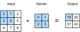
Convolutional layer. Instead of connecting every pixel to every neuron (a dense layer), a convolutional layer slides a small learned filter — say 5×5 numbers — across the image and, at each position, multiplies and sums the overlapping values into one output cell. The same filter is reused at every position, so the layer learns local patterns (an edge, a corner, a stroke) wherever they appear, with a few dozen weights instead of millions (LeCun, Bottou, Bengio & Haffner, 1998, "Gradient-Based Learning Applied to Document Recognition", Proc. IEEE; the mechanism dates to Fukushima's neocognitron, 1980). One layer learns many filters; each produces its own output map ("channel"):
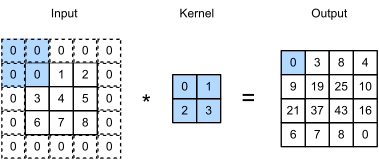
Padding. Each pass of a filter shrinks the image (a 5×5 filter turns
28×28 into 24×24) and reads border pixels fewer times than central ones.
Padding fixes both: rows and columns of zeros around the input let the
filter's center reach the true edges, so the output keeps the input's size
(pad=1 with 3×3 filters — the VGG recipe) and border information
survives deep stacks. The full input/output-size arithmetic is worked out
in Dumoulin & Visin (2016), "A guide to convolution arithmetic for deep
learning", arXiv:1603.07285:
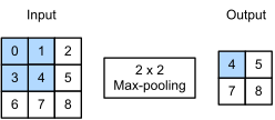
Max pooling. Between convolutions, a pooling layer slides a small window (here 2×2) and keeps only the largest value in it — the image halves in width and height, the strongest responses survive, and the exact pixel position of a feature stops mattering (a slightly shifted "7" is still a "7"). Max beats average pooling for recognition in the systematic comparison of Scherer, Müller & Behnke (2010, "Evaluation of Pooling Operations in Convolutional Architectures for Object Recognition", ICANN):
Stack these — convolve, pool, convolve, pool, then a couple of dense layers — and you have every model in the zoo below.
Concept diagrams by Zhang, Lipton, Li & Smola, Dive into Deep Learning, CC BY-SA 4.0, unmodified — the same source and license as the architecture diagrams below.
Model zoo
Honest names: these are the classic architectures at small-image scale, not the ImageNet originals.
| model | architecture | paper |
|---|---|---|
lenet5 |
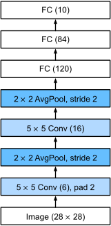
Conv 6@5x5 → pool → Conv 16@5x5 → pool → 120 → 84 → classes; faithful C1..F6 shapes (relu instead of the paper's tanh — flagged deviation) | LeCun, Bottou, Bengio & Haffner (1998), "Gradient-Based Learning Applied to Document Recognition", Proc. IEEE 86(11) |
minivgg |
[32, 32, pool] → [64, 64, pool] → 128 → classes, all 3x3 pad-1 — VGG-style blocks at CIFAR scale, not VGG-16 | Simonyan & Zisserman (2015), "Very Deep Convolutional Networks for Large-Scale Image Recognition", ICLR |
alexnet_small |
64 → pool → 192 → pool → 384 → 256 → 256 → pool → 1024 → 512 → classes, 3x3 kernels — AlexNet-style at CIFAR scale, not the ImageNet net | Krizhevsky, Sutskever & Hinton (2012), "ImageNet Classification with Deep Convolutional Neural Networks", NeurIPS |
The originals, for reference
What the papers built (our zoo keeps the layer pattern and shrinks the scale — see the honest-name notes above):
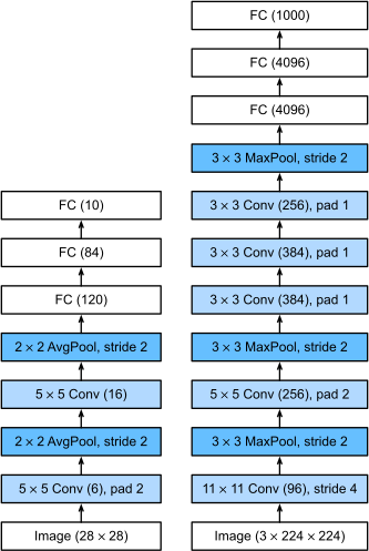
LeNet-5 (LeCun et al., 1998) — lenet5 keeps these exact C1..F6 shapes:
AlexNet (Krizhevsky et al., 2012) vs LeNet — alexnet_small keeps the
conv-conv-conv stack and the big dense head, at 32×32:
VGG (Simonyan & Zisserman, 2015) — minivgg keeps the same-width 3×3
conv blocks with pooling between, two blocks instead of five:
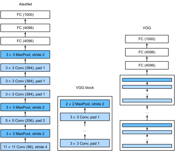
Diagrams by Zhang, Lipton, Li & Smola, Dive into Deep Learning (LeNet-5 and AlexNet via Wikimedia Commons), licensed CC BY-SA 4.0 — redistributed here with attribution, unmodified.
Datasets
Five image-classification classics plus one from particle physics.
Nothing downloads implicitly — data/ is gitignored and library code
never touches the network; missing files raise with the exact fix command.
| name | train/test | shape | classes | source |
|---|---|---|---|---|
| mnist | 60k / 10k | 1×28×28 | 10 | LeCun et al. (1998) |
| fashion_mnist | 60k / 10k | 1×28×28 | 10 | Xiao, Rasul & Vollgraf (2017) |
| kmnist | 60k / 10k | 1×28×28 | 10 | Clanuwat et al. (2018) |
| qmnist | 60k / 60k | 1×28×28 | 10 | Yadav & Bottou (2019) |
| cifar10 | 50k / 10k | 3×32×32 | 10 | Krizhevsky (2009) |
| atlas_calo | ~190k / ~48k | 1×24×24 | 2 | ATLAS Collab. (2021) — CERN Open Data 15012, CC0, DOI |
One test sample from each, with a LeNet-5's output under it (3-epoch protocol budget; correctly-classified examples — the measured accuracy per dataset is in Results):
| mnist | fashion_mnist | kmnist | cifar10 | qmnist | atlas_calo |
|---|---|---|---|---|---|
 |
 |
 |
 |
 |
 |
| → “4” | → “t-shirt” | → “na” (な) | → “airplane” | → “2” | → “photon” |
The last is not a photo: it is a calorimeter shower rendered as a
(depth × radius) energy map — see below. datasets.load(name) →
(X_train, y_train, X_test, y_test), NCHW float32 in [0, 1], int32 labels.
datasets.subset(name, n_train, n_test, seed) gives seeded stratified
subsets (the benchmark protocol uses 2000/1000).
A CERN dataset in the zoo
atlas_calo is real detector physics, from the CERN Open Data
Portal (record 15012, CC0). When a
particle from an LHC collision enters the ATLAS calorimeter it showers — it
splits into a cascade of secondary particles that deposits its energy across
the calorimeter's ~24 concentric sampling layers. How it showers betrays
what it is: a photon showers electromagnetically, a compact cascade
that dumps its energy in the first few layers; a charged pion showers
hadronically, a broader cascade that punches deep into the later layers.
Telling the two apart from shower shape is a genuine ATLAS task — here, a
two-class image problem.
The record ships each shower as a flat list of per-voxel energies (the ATLAS
AtlFast3 fast-simulation GAN training
samples — Aad et al., Comput. Softw. Big Sci. 6, 7, 2022). But the
voxels are spatial: each has a radius r and azimuth α within its layer.
The loader averages over α (showers are ~azimuthally symmetric) and regrids
each layer's radial bins onto a common axis, producing a (24 layer × 24
radius) energy map — depth down the rows, lateral spread across the
columns. Photons light the top (electromagnetic) rows; pions also light the
deep (hadronic) rows. That is exactly the local, translation-shared spatial
structure a convolution is built to read — a CNN honestly fits here, not by
analogy to photographs but because a shower is a 2-D pattern of energy. One
channel: this record stores energy only (the CMS ECAL image sets add a timing
channel); a fabricated second channel would be dishonest.
Results
Protocol: the same architecture, re-expressed layer-for-layer in each
framework (torch.nn.Sequential, tf.keras.Sequential, our Sequential),
identical hyperparameters everywhere — plain SGD, lr 0.01, batch 32, 3
epochs, seed 0 — on stratified 2000-train / 1000-test subsets, CPU only.
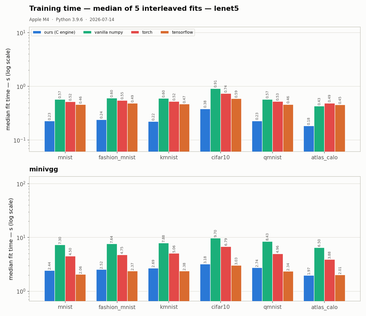
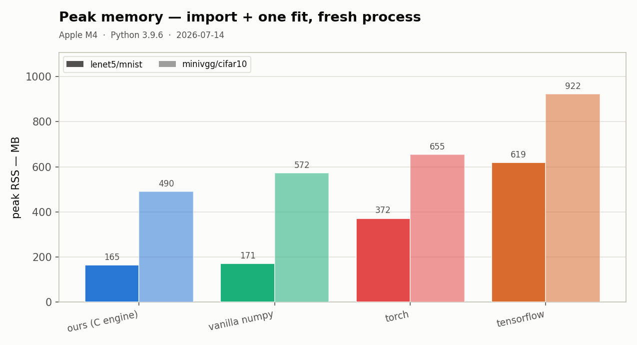
Fit wall-time is the median of 5 interleaved repeats; peak RSS is one fresh
subprocess per (contender, pair), import cost included. vanilla numpy is
this package's pure-numpy reference backend — no mantissa engine — showing
what the C core buys. scikit-learn is deliberately absent: it offers no
convolutional layers, so it cannot run these architectures.
LeNet-5 on MNIST (28×28 grayscale — the architecture's home ground):
| contender | fit (s) ↓ | predict (ms) ↓ | peak RSS (MB) ↓ | test acc |
|---|---|---|---|---|
| ours (mantissa) | 0.228 | 8.1 | 165 | 0.782 |
| tensorflow | 0.458 | 42.1 | 619 | 0.846 |
| torch | 0.519 | 13.4 | 372 | 0.762 |
| vanilla numpy | 0.575 | 40.0 | 171 | 0.782 |
Mini-VGG on CIFAR-10 (32×32 RGB — the heavy, 3×3-block workload):
| contender | fit (s) ↓ | predict (ms) ↓ | peak RSS (MB) ↓ | test acc |
|---|---|---|---|---|
| tensorflow | 3.027 | 165.6 | 922 | 0.187 |
| ours (mantissa) | 3.182 | 175.2 | 490 | 0.292 |
| torch | 6.789 | 256.6 | 655 | 0.288 |
| vanilla numpy | 9.696 | 608.5 | 572 | 0.294 |
The honest read.
- LeNet-scale nets are ours across the board: on all five datasets the C engine fits ~1.5–2.4× faster than torch and tensorflow (torch 1.9–2.4×, tensorflow 1.5–2.1× behind), runs the fastest batch predict, and holds the lowest peak RSS (2.3–3.8× under the frameworks on MNIST). At this scale the frameworks pay per-op dispatch and graph overhead that a thin C core simply doesn't have.
- The heavy VGG blocks are a photo finish: the first run of this table had TensorFlow's compiled graph 1.3× ahead on minivgg fit and 1.6× on predict. That gap was recorded as the engine's next target, and mantissa v0.2.2 (batch-whole panel-packed GEMM + a NEON 6×16 micro-kernel, 148 → 363 GFLOP/s on the VGG-block shape) closed it to single digits. Re-measured under v0.2.3, TensorFlow leads by 5% on fit and 6% on predict on CIFAR-10 (5–18% on fit across the five VGG pairs — gaps this small move between runs about as much as between releases) — while ours uses 47% less peak memory than TensorFlow. torch's eager mode trails ours 2.1× here. The remainder is Winograd territory, and it is recorded as such.
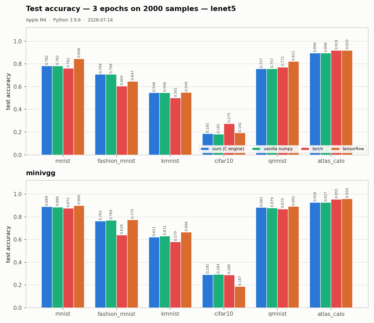
- Accuracy lands in the same band for everyone on each pair — same structure, same budget, different init/shuffle streams (seeded per framework; they cannot be made bit-identical across libraries). Nobody tuned anything. CIFAR-10 at 2000 samples × 3 epochs is hard for every contender (0.19–0.30) — that row measures speed under a fixed budget, not achievable CIFAR accuracy.
- The benchmark improved the package: the first RSS pass was dominated
by dataset loading in every contender —
load()converted the full set to float32 beforesubset()sliced it. Loading now stays uint8 until after the slice (bit-identical subsets, measured 672 → 195 MB on the qmnist worker). Measure, don't assume. - The physics dataset behaves like a dataset, not a gimmick. On
atlas_calo(24×24 single-channel shower maps, 2 classes) ours leads both pairs outright: lenet5 fit 0.185 s vs tensorflow 0.454, vanilla numpy 0.429, torch 0.487 (predict 6.1 ms vs 9.6–41.6 ms); minivgg fit 1.966 s vs tensorflow 2.006, torch 3.878, vanilla numpy 6.497 (predict 92.6 ms vs 104.7–341.6 ms) — with the lowest peak RSS on both (99–100 MB vs 256–592 MB for the frameworks; the memory-mapped voxel subset load keeps every worker lean, ours leanest). Test accuracy under the fixed 3-epoch/2000-sample budget is 0.896–0.959 across contenders (ours 0.896 lenet5 / 0.926 minivgg) — well above the 0.5 coin-flip and the 0.79 the best single total-hadronic-energy threshold achieves on the same subset, so the nets are reading shower shape, not one summary number.
Fairness caveats. TF's one-time graph tracing is excluded from fit
timing (as imports are for everyone); torch runs eager, its default mode.
CPU only — no MPS/Metal on any contender. Thread settings left at each
framework's defaults and recorded in the JSON. All raw samples live in
bench/results/ (regenerable, gitignored).
Environment. Apple M4 · Python 3.9.6 · numpy 2.0.2 · torch 2.8.0 ·
tensorflow 2.20.0 · mantissa 0.2.3 (f32 CNN primitives, audit release) ·
2026-07-14.
Protocol note (v0.2.0): the two atlas_calo pairs were added later and
measured 2026-07-16 — same machine, versions and protocol, different day
(recorded as env.atlas_calo_date in the results JSONs); the five original
datasets' numbers above are the untouched 2026-07-14 run.
Reproduce: python -m bench.speed && python -m bench.accuracy && python -m bench.plots.
Methodology
Fixed protocol for every contender: identical architectures, subsets, epochs, batch size, learning rate and seeds. Timings are medians over interleaved repeats on one machine (library versions and CPU recorded in the results JSON); peak RSS is measured per contender in a fresh subprocess, import cost included, because that is what a user pays. scikit-learn cannot express a CNN, so its MLP entry is labeled a non-CNN baseline, not a rival. Measure, don't assume.
License
MIT — © Tekin Ertekin. Engine: mantissa, same author, MIT.
1 maintainer

Metadata
1 maintainer
Release files for mantissa-cnn 0.2.2
For a detailed explanation of source distributions (sdists) and built distributions (wheels), please see the package formats documentation.
Source distribution (sdist)
| File | Size | Uploaded | Provenance | |
|---|---|---|---|---|
| mantissa_cnn-0.2.2.tar.gz | 40.5 kB | With provenance | Details |
Built distribution (wheel)
| File | Interpreter | ABI | Platform | Reset |
|---|---|---|---|---|
| mantissa_cnn-0.2.2-py3-none-any.whl | Python 3 | none | any | Details |
Total release size: 69.0 kB
Release files / mantissa_cnn-0.2.2.tar.gz
| Download URL | mantissa_cnn-0.2.2.tar.gz |
|---|---|
| Size | 40.5 kB |
| Tags | Source |
|
SHA-256 checksum How to use checksums |
6d9a063581ec8851ca8edfe93bcf298a80d21b79b7bed331e3482f9335164d17
|
|
BLAKE2b-256 checksum How to use checksums |
1b1de006a6ccd2b57cc0b9bed0cf63e2d47b618d0d2cdaf1caad8d7caf52a8c8
|
| Upload date | |
|
Uploaded using Trusted Publishing? What is trusted publishing? |
Yes |
| Uploaded via |
twine/6.1.0 CPython/3.13.12
|
Provenance
Provenance describes where a file came from. On PyPI, provenance is shared via attestations, which provide a verifiable record of the build or publishing details. View details, limitations and caveats.


PyPI Publish Attestation
PyPI verified that this artifact, at this checksum, originated from the publisher listed below.
Signed by GitHub Actions, verified by PyPI on Jul 19, 2026.
Transparency logRelease files / mantissa_cnn-0.2.2-py3-none-any.whl
| Download URL | mantissa_cnn-0.2.2-py3-none-any.whl |
|---|---|
| Size | 28.5 kB |
| Tags | Python 3 |
|
SHA-256 checksum How to use checksums |
cc7908817c4f52f5bc3e2a4f511db5e847e7a8dbee690a9610a198faf3daccad
|
|
BLAKE2b-256 checksum How to use checksums |
2c4fc049b6fea952848c7a8d013f004f7e5ba2c74582bf5c0e397f0087ffb9c2
|
| Upload date | |
|
Uploaded using Trusted Publishing? What is trusted publishing? |
Yes |
| Uploaded via |
twine/6.1.0 CPython/3.13.12
|
Provenance
Provenance describes where a file came from. On PyPI, provenance is shared via attestations, which provide a verifiable record of the build or publishing details. View details, limitations and caveats.
PyPI Publish Attestation
PyPI verified that this artifact, at this checksum, originated from the publisher listed below.
Signed by GitHub Actions, verified by PyPI on Jul 19, 2026.
Transparency logSecurity for mantissa-cnn 0.2.2
Provenance
Provenance describes where a file came from. On PyPI, provenance is shared via attestations, which provide a verifiable record of the build or publishing details. View details, limitations and caveats.
Full provenance
All 2 files in this release have been uploaded with provenance metadata.
Attestation for mantissa_cnn-0.2.2.tar.gz
PyPI Publish Attestation
PyPI verified that this artifact, at this checksum, originated from the publisher listed below.
Signed by GitHub Actions, verified by PyPI on Jul 19, 2026.
Transparency logA note on package security
PyPI is a repository for distributing packages, not a service for auditing them. While third-party security researchers and our staff do their best to detect and remove malicious packages, PyPI cannot guarantee the quality, security or suitability of any given package.
To learn more about protecting yourself from malicious actors, visit our package security documentation.














