
mantissa-interpret




Seeing what a CNN looks at. A trained classifier gives you a label; it does
not tell you why. mantissa-interpret answers that with three classic
attribution methods that turn a prediction into a heatmap over the input —
bright where the pixels mattered for the class, dark where they did not.
Everything runs on a fitted mantissa_cnn.Sequential
model, using the model's own forward and backward passes through the mantissa
C engine — the same engine it was trained on. There is no PyTorch/TensorFlow
dependency: the heatmaps come out of the same low-precision C kernels that
produced the prediction.
The mantissa family
Part of the mantissa family: a low-precision engine written in C, with small Python packages built on top. Each package sits under the one it depends on — ⭐ marks where you are, and every other name links to its repo.
- mantissa — low-precision neural-network engine in C (the core)
- mantissa-perceptron — perceptron & ADALINE, the linear classics
- mantissa-nn — shared neural-net primitives (layers, engine binding)
- mantissa-cnn — convolutional networks for images
- mantissa-auto-encoder — autoencoders for denoising & super-resolution
- ⭐ mantissa-interpret — CNN interpretability (occlusion, saliency, Grad-CAM) (you are here)
- mantissa-embed — CNN metric learning (image embeddings for similarity & retrieval)
- mantissa-mlp — multilayer perceptrons, fully-connected nets
- mantissa-cnn — convolutional networks for images
New to interpretability?
A CNN classifier turns an image into a label — but the label alone hides why. Interpretability (here, attribution) recovers the missing reason: it marks which parts of the input the model actually used for a given class, as a heatmap laid over the image. That matters because a model can be right for the wrong reason — keying on a watermark, a background, or a dataset artifact instead of the object — and a bare accuracy number will never tell you. A heatmap will.
The most direct way to see this is to hide part of the image and watch the prediction. If covering a region makes the class probability collapse, that region carried the evidence; if nothing changes, it did not:
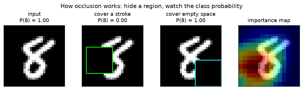
That single experiment is the first method. The three methods here are three answers to "what did the model use?", trading detail for cost and clarity:
- Occlusion — exactly the picture above, done everywhere: slide a patch over the image and record how much each position, when hidden, drops the class probability. No math beyond running the model forward; the price is one forward pass per patch, and the resolution is patch-sized.
- Saliency — instead of hiding pixels, ask calculus which pixels matter: the gradient of the class score with respect to each input pixel. A large gradient means "nudging this pixel would move the score a lot." It is per-pixel sharp but noisy, and needs a single backward pass.
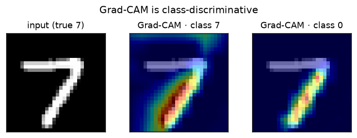
- Grad-CAM — work inside the network. At a convolutional layer each channel is a learned feature detector over a coarse grid; weight every channel by how much raising its activation would raise the target score (its gradient), add them up, and keep the positive part. The result is a smooth, class-discriminative region — ask about "3" vs "7" on the same image and the map moves — for one backward pass.
Occlusion and saliency answer which pixels; Grad-CAM answers which region, for this class. Together they are the standard first tools for debugging a model that is right for the wrong reason.
Install
pip install mantissa-interpret
Pulls in mantissa-cnn (and transitively mantissa-nn + the mantissa-core
engine). For plotting the heatmaps, pip install mantissa-interpret[viz].
The three methods
| method | cost | granularity | class-discriminative | needs |
|---|---|---|---|---|
occlusion_map |
forward only, O(patches) | coarse (patch) | yes | — |
saliency_map |
one backward pass | per-pixel (noisy) | weakly | input gradient |
grad_cam |
one backward pass | per-region (smooth) | yes | activations + their gradient at a conv layer |
Each takes a fitted model and a single (C, H, W) image and returns a 2-D
heatmap normalized to [0, 1], aligned to the input.
Occlusion — occlusion_map
Slide a patch×patch window (filled with fill) across the image; at each
position, hide that window and re-run the model. If the target class
probability drops a lot, those pixels were important. The heatmap is the
per-pixel average drop (overlapping windows blend), normalized to [0, 1].
from mantissa_interpret import occlusion_map
heat = occlusion_map(net, image, target_class=7, patch=7, stride=3)
Only forward passes — model-agnostic and dead simple, but coarse (patch-sized) and its cost scales with the number of windows. All occluded copies are run in a single batched forward pass.
Saliency — saliency_map
The first-order sensitivity of the class score to each pixel is just its
gradient. One forward pass primes the layers, we seed the gradient of the
target logit (a one-hot vector), and backpropagate to the input — the same
backward the model trains with, carried one step past the first layer's
weights down to the pixels. The map is |gradient| reduced over channels.
from mantissa_interpret import saliency_map
heat = saliency_map(net, image, target_class=7)
Per-pixel and cheap (one backward pass), but high-frequency and noisy, and only weakly class-discriminative — good for "which strokes", not "which region".
Grad-CAM — grad_cam
At a convolutional layer, each channel is a learned feature detector over a coarse grid. Grad-CAM weights every channel by the average gradient of the target logit w.r.t. that channel's activation (how much "more of this feature" raises the class score), sums the channels with those weights, keeps the positive part, and upsamples to the image. We capture the layer's activation on the forward pass and backpropagate the logit down to that same layer for the gradient — then combine.
from mantissa_interpret import grad_cam
heat = grad_cam(net, image, target_class=7)      # last Conv2D by default
Coarse (conv-grid resolution) but smooth and genuinely class-discriminative
— asking about different classes on the same image yields different maps.
target_layer selects which conv layer to read (default: the last one).
Results
A LeNet-5 trained on an 8k-image MNIST subset with the mantissa C engine
(3 epochs, 96% test accuracy), then explained on held-out digits. Reproduce
with python examples/heatmaps_demo.py.
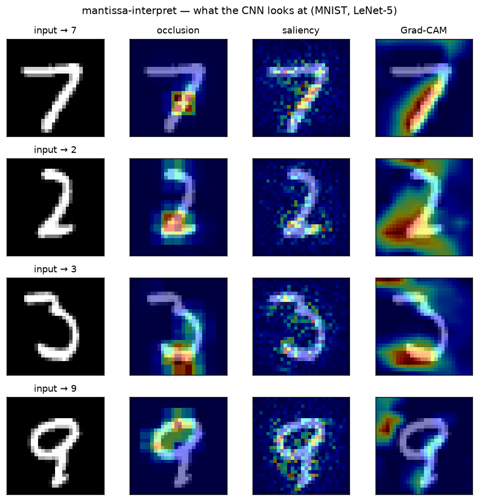
Reading across a row, the three methods agree on the digit but differ exactly as their math predicts:
- occlusion — coarse, patch-sized blobs on the strokes whose removal costs the class the most;
- saliency — the finest detail, tracing individual strokes, but visibly noisy (the raw per-pixel gradient);
- Grad-CAM — a smooth region over the class-defining strokes (the 7's diagonal, the 2's base, the 9's loop), with the least clutter.
Grad-CAM is also class-discriminative — ask it about a different target class on the same image and the map moves:
All of this — feature maps, gradients, the optimization-free attribution — comes out of the same low-precision C kernels the model was trained on.
License
MIT — Tekin Ertekin.
1 maintainer

Download files
Download the file for your platform. If you're not sure which to choose, learn more about installing packages.
Source Distribution
Built Distribution
Filter files by name, interpreter, ABI, and platform.
If you're not sure about the file name format, learn more about wheel file names.
Copy a direct link to the current filters
File details
Details for the file mantissa_interpret-0.1.0.tar.gz.
File metadata
- Download URL: mantissa_interpret-0.1.0.tar.gz
- Upload date:
- Size: 9.5 kB
- Tags: Source
- Uploaded using Trusted Publishing? Yes
- Uploaded via:
twine/6.1.0 CPython/3.13.14
File hashes
| Algorithm | Hash digest | |
|---|---|---|
| SHA256 |
4d999d93519be5bea6e6c32bd88030d480eed38027e3ca22515c7a00805ab7ef
|
|
| MD5 |
45c4ed05d36e68db7d4183f5bb5aca15
|
|
| BLAKE2b-256 |
c50de6402f6deed2a8514ef0a546a7801d0cab2ed1f495ab81982bc50708d5cc
|
Provenance
The following attestation bundles were made for mantissa_interpret-0.1.0.tar.gz:
Publisher:
release.yml on tekinertekin/mantissa-interpret
-
Statement:
-
Statement type:
https://in-toto.io/Statement/v1 -
Predicate type:
https://docs.pypi.org/attestations/publish/v1 -
Subject name:
mantissa_interpret-0.1.0.tar.gz -
Subject digest:
4d999d93519be5bea6e6c32bd88030d480eed38027e3ca22515c7a00805ab7ef - Sigstore transparency entry: 2248991593
- Sigstore integration time:
-
Permalink:
tekinertekin/mantissa-interpret@2bdc557dfe897d0f7f04880e0f3c90379c5e35b2 -
Branch / Tag:
refs/tags/v0.1.0 - Owner: https://github.com/tekinertekin
-
Access:
public
-
Token Issuer:
https://token.actions.githubusercontent.com -
Runner Environment:
github-hosted -
Publication workflow:
release.yml@2bdc557dfe897d0f7f04880e0f3c90379c5e35b2 -
Trigger Event:
push
-
Statement type:
File details
Details for the file mantissa_interpret-0.1.0-py3-none-any.whl.
File metadata
- Download URL: mantissa_interpret-0.1.0-py3-none-any.whl
- Upload date:
- Size: 11.3 kB
- Tags: Python 3
- Uploaded using Trusted Publishing? Yes
- Uploaded via:
twine/6.1.0 CPython/3.13.14
File hashes
| Algorithm | Hash digest | |
|---|---|---|
| SHA256 |
1f778262f92a7f20cc75b35300401306b8d3d328e628ab6e7ec7274933c1ec0f
|
|
| MD5 |
162f084c0569c27096e2b53c082178a8
|
|
| BLAKE2b-256 |
1b9b64cc76fbdd3b9a418e83303d8a858ec0a00d63931cb54c9d12775786b2a0
|
Provenance
The following attestation bundles were made for mantissa_interpret-0.1.0-py3-none-any.whl:
Publisher:
release.yml on tekinertekin/mantissa-interpret
-
Statement:
-
Statement type:
https://in-toto.io/Statement/v1 -
Predicate type:
https://docs.pypi.org/attestations/publish/v1 -
Subject name:
mantissa_interpret-0.1.0-py3-none-any.whl -
Subject digest:
1f778262f92a7f20cc75b35300401306b8d3d328e628ab6e7ec7274933c1ec0f - Sigstore transparency entry: 2248992019
- Sigstore integration time:
-
Permalink:
tekinertekin/mantissa-interpret@2bdc557dfe897d0f7f04880e0f3c90379c5e35b2 -
Branch / Tag:
refs/tags/v0.1.0 - Owner: https://github.com/tekinertekin
-
Access:
public
-
Token Issuer:
https://token.actions.githubusercontent.com -
Runner Environment:
github-hosted -
Publication workflow:
release.yml@2bdc557dfe897d0f7f04880e0f3c90379c5e35b2 -
Trigger Event:
push
-
Statement type:













