
mantissa-mlp




The multilayer perceptron, with a C engine.
An MLP classifier for tabular data (fit / predict / predict_proba /
score) built on top of
mantissa-cnn: its Dense
layer, its mantissa C-engine and
pure-numpy backends, and its fused softmax-cross-entropy loss are all
reused, not reimplemented. This package adds what tabular classification
needs on top of that: the (n, d) training loop, a small cited zoo, six
tabular datasets — two of them published by CERN, including the ATLAS
Higgs challenge set — and the AMS physics metric the challenge was actually
scored with.
This repo is also the resolution of a cliffhanger. The family's first
package, mantissa-perceptron,
ends its concept section at Minsky & Papert's famous limit: a single neuron
draws a single line, so it can never represent XOR. The fix promised there —
a hidden layer between input and output, trained by backpropagation — is
this package. models.xor_net() is twelve numbers that end a
half-century-old argument.
Deliberately minimal, like the rest of the family: float32 features, integer class ids, softmax cross-entropy (binary is the 2-class case), plain SGD. No autograd graph, no optimizer zoo, no early stopping. Layers allocate their scratch once per batch shape and reuse it — steady-state training does no per-batch allocation.
Install
pip install mantissa-mlp
This pulls in mantissa-cnn >= 0.1.0 (which pulls the engine
mantissa-core >= 0.2.1).
From checkouts (works today, no PyPI needed): clone this repo, cnn, and
mantissa side by side, build the
engine (make dist there), then here:
pip install -e ../cnn && pip install -e ".[dev]"
mantissa-cnn finds the sibling engine checkout automatically; this package
finds mantissa-cnn's data/ (for mnist_flat) and a sibling
mantissa-perceptron checkout's banknote file automatically.
Quickstart
# datasets never download implicitly — fetch explicitly, once (~62 MB):
python -m mantissa_mlp.datasets download higgsml
python -m mantissa_mlp.datasets list
from mantissa_mlp import models, datasets, tasks

Xtr, ytr, wtr, Xte, yte, wte = datasets.load("higgsml", weights=True)
Xtr, Xte = tasks.standardize(Xtr, Xte, missing=-999.0)   # sentinel-aware

net = models.higgs_mlp()                 # C engine; backend="numpy" also works
print(net.summary())
net.fit(Xtr, ytr, epochs=5, batch_size=32, lr=0.01, verbose=True)
print("accuracy:", net.score(Xte, yte))
print("AMS     :", tasks.ams(yte, net.predict(Xte), wte))   # the physics metric
And the twelve-number family story:
import numpy as np
from mantissa_mlp import models

X = np.array([[0, 0], [0, 1], [1, 0], [1, 1]], dtype=np.float32)
y = np.array([0, 1, 1, 0], dtype=np.int32)
net = models.xor_net()
net.fit(X, y, epochs=500, batch_size=1, lr=0.3)   # per-pattern, as in 1986
print(net.score(X, y))                            # 1.0
Or compose your own:
from mantissa_mlp import MLP

net = MLP(hidden=(64, 32), act="relu", classes=7, seed=0)
New to MLPs? The three ideas in this package
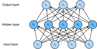
The hidden layer. A single neuron computes step(w·x + b) — one
learned line through feature space. Minsky & Papert (Perceptrons, MIT
Press, 1969) made precise what that excludes: no line puts XOR's (0,0) and
(1,1) on one side and (0,1) and (1,0) on the other, and the finding froze
neural-network research for a decade. The fix is not a better line but a
layer of neurons between input and output: each hidden unit draws its own
line, and the output unit combines their verdicts — two half-planes AND-ed
and OR-ed into a band that XOR fits inside. Width buys expressiveness:
Backpropagation. Hidden layers were proposed long before anyone could
train them — the credit-assignment problem: how much of the output error is
hidden unit 3's fault? Rumelhart, Hinton & Williams (1986, "Learning
representations by back-propagating errors", Nature 323) gave the answer
that stuck: run the chain rule backwards. The forward pass computes each
layer's output; the backward pass propagates ∂loss/∂output from the top
layer down, each layer multiplying by its local derivative, so every weight
in every layer gets an exact gradient in one backward sweep that costs about
as much as the forward one. XOR is that paper's first worked example, and
models.xor_net() reproduces it: per-pattern updates, one hidden layer,
the whole net converging to all four corners. (This package's test suite
verifies the backward sweep against finite differences through two hidden
layers — trust, but differentiate.)
Universal approximation. One hidden layer is not just enough for XOR. Cybenko (1989, "Approximation by Superpositions of a Sigmoidal Function", Mathematics of Control, Signals and Systems 2(4)) proved that a single hidden layer of sigmoidal units, wide enough, approximates any continuous function on a compact set to any accuracy; Hornik (1991, "Approximation capabilities of multilayer feedforward networks", Neural Networks 4(2)) showed it is the layered structure, not the particular activation, that matters. That is the license behind applying one architecture family to detector physics, forests, wine and banknotes below — and the theorem says nothing about finding the weights, which is why the training loop and its budget are what this family actually measures.
Concept diagram by Zhang, Lipton, Li & Smola, Dive into Deep Learning, licensed CC BY-SA 4.0 — redistributed here with attribution, unmodified. The same figure, source and license as the sister repo mantissa-perceptron's concept section, where it is the promised fix; here it is the package.
The CERN datasets: where they come from
Two of the six datasets below are not UCI classics but genuine particle-physics data products, published by CERN on its Open Data portal — one from each of the LHC's two general-purpose experiments. They deserve their origin story.
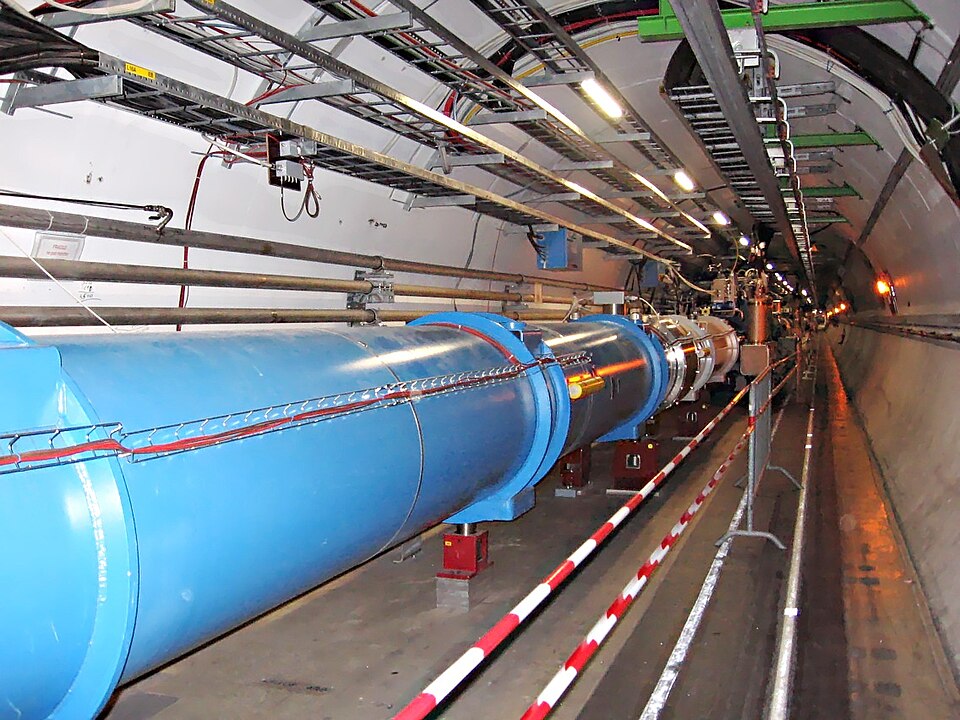
The machine. The Large Hadron Collider accelerates two beams of protons to 99.999999% of light speed around a 27 km ring under the Franco-Swiss border and crosses them at four points, hundreds of millions of collisions per second:
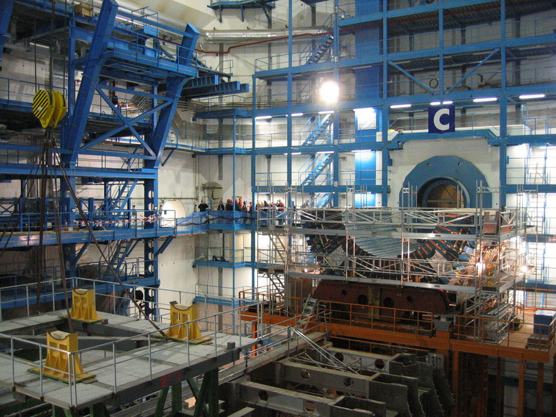
The detectors. At the crossing points sit cathedral-sized instruments — ATLAS (46 m long, 7000 t) and CMS are the two general-purpose ones — that photograph each collision's debris: silicon trackers record charged-particle paths, calorimeters absorb and measure energy, muon chambers catch what punches through everything else:
higgsml — the ATLAS Higgs challenge (record 328)
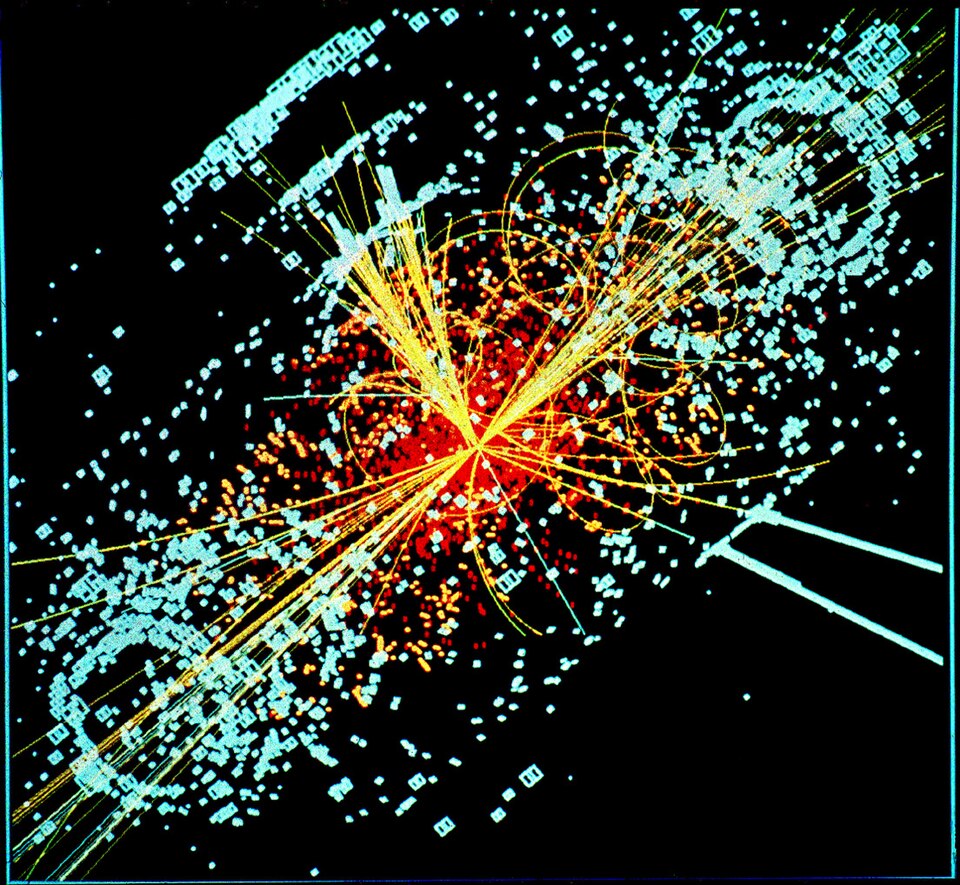
After the 2012 Higgs discovery, the harder question was whether the new boson decays to fermions as the Standard Model demands. The H → τ⁺τ⁻ channel was the frontier: a faint signal buried under Z → ττ decays that look nearly identical. In 2014 the ATLAS collaboration turned that exact analysis into the Higgs Boson Machine Learning Challenge (1785 teams — then Kaggle's largest), and afterwards published the full 818,238 simulated events on the CERN Open Data portal as record 328 (CC0, DOI 10.7483/OPENDATA.ATLAS.ZBP2.M5T8) — official ATLAS simulation, the detector response and all:
- The 30 features come in two families, named honestly in the file:
PRI_*(primitives — quantities the detector measures more or less directly: lepton momenta, missing transverse energy, jet four-vectors) andDER_*(derived — quantities ATLAS physicists computed from the primitives because decades of analysis say they discriminate: invariant masses, angular separations, centralities). Feeding both to a model asks it to match hand-crafted physics insight; the related deep-learning result of Baldi, Sadowski & Whiteson (2014, "Searching for exotic particles in high-energy physics with deep learning", Nature Communications 5:4308) is that deep networks can recover much of theDER_*information from primitives alone. - -999.0 means "does not exist", not "not measured": jet-dependent
variables are undefined when the event has fewer jets than the formula
needs (
DER_mass_jet_jetneeds two jets), andDER_mass_MMCis undefined when the mass fitter fails. The challenge documentation (Adam-Bourdarios et al. 2015, appendix B) fixed the sentinel at −999.0, outside every physical range. This package's documented handling lives intasks.standardize(missing=-999.0): sentinels are excluded from the train statistics, then imputed as 0.0 — the post-standardization mean, exactly neutral to a Dense layer's weighted sum. - AMS, not accuracy. Unweighted, the simulation is ~⅓ signal; reality
is not — each event carries a weight renormalizing simulation to
real detector rates, where the signal is vanishingly rare. The challenge
metric is the Approximate Median Significance,
AMS = sqrt(2·((s+b+10)·ln(1+s/(b+10)) − s))withs,bthe summed weights of selected signal and background: the median number of Gaussian sigmas with which the selection would establish that the signal exists. A high-accuracy classifier can still be a poor discovery instrument;tasks.ams()is the exact section-3 formula, and the loaders keep the weights renormalized per split so the numbers stay comparable to the challenge's own (~3.8 winning score).
dimuon — the CMS dimuon spectrum (record 545)
The other general-purpose experiment, CMS, published a classic teaching dataset: 100,000 real (not simulated) events from 2011 in which the detector saw two muons, with each muon's energy, momentum vector, and charge (record 545, CC0; McCauley, 2017). Histogram the invariant mass of the pair and half a century of physics appears as peaks on a falling background: the J/ψ at 3.10 GeV (1974, charm quark), the Υ family at 9.5–10.4 GeV (1977, bottom quark), the Z at 91 GeV (1983, electroweak unification).
The task this package builds from it: predict which resonance an event
belongs to from the muon kinematics — 16 features (E, p_x, p_y, p_z, p_T, η, φ,
charge, per muon), 3 classes. The labels are constructed, and honestly
so: an event is labeled J/ψ, Υ or Z by which invariant-mass window
(2.8–3.4, 9.0–11.0, 60–120 GeV) it falls in, off-peak events are dropped
(26,911 of the 100,000 remain — measured: 8,628 J/ψ, 12,159 Υ, 6,124 Z),
and the mass itself is excluded from the features. Since the mass is a
closed-form function of the features (M² = (E₁+E₂)² − |p₁+p₂|²), the
task is learnable by construction — what it measures is whether a small
MLP can approximate that nonlinear function well enough to separate
three mass scales, which is the universal-approximation section above
made concrete on real detector data.
Photographs and event display via Wikimedia Commons, licenses verified on each file page: LHC tunnel by Julian Herzog, CC BY-SA 3.0, scaled to 960 px; ATLAS cavern by Nikolai Schwerg, CC BY-SA 3.0, unmodified; simulated CMS Higgs event by Lucas Taylor / CERN, CC BY-SA 3.0, scaled to 960 px — all redistributed here with attribution.
Papers: Adam-Bourdarios, Cowan, Germain, Guyon, Kégl & Rousseau (2015), "The Higgs boson machine learning challenge", JMLR W&CP 42; ATLAS Collaboration (2014), dataset DOI 10.7483/OPENDATA.ATLAS.ZBP2.M5T8; McCauley (2017), CERN Open Data record 545; Baldi, Sadowski & Whiteson (2014), Nature Communications 5:4308.
Model zoo
Honest names: cited recipes at this package's scale, deviations flagged in each docstring.
| model | architecture | paper |
|---|---|---|
xor_net |
2 → 2 tanh → 2 logits — the minimal hidden-layer net; the paper's 2-2-1 with the family's softmax head instead of one sigmoid unit (flagged), per-pattern training recipe in the docstring | Rumelhart, Hinton & Williams (1986), "Learning representations by back-propagating errors", Nature 323; Cybenko (1989), MCSS 2(4) |
tabular_mlp |
d → 64 → 32 → classes, relu — the generic workhorse | Rumelhart, Hinton & Williams (1986); the default shape is the modern textbook baseline (Goodfellow, Bengio & Courville, 2016, ch. 6) |
higgs_mlp |
30 → 300 → 200 → 100 → 2, relu — 600 hidden units in the spirit of the HiggsML winners' nets; no ensemble, no momentum/dropout (flagged) | Adam-Bourdarios et al. (2015), "The Higgs boson machine learning challenge", JMLR W&CP 42 |
Datasets
Six tabular classification sets. Nothing downloads implicitly —
data/ is gitignored and library code never touches the network; missing
files raise with the exact fix command:
python -m mantissa_mlp.datasets download <name|all>
python -m mantissa_mlp.datasets list
| name | train/test | d | classes | task | source |
|---|---|---|---|---|---|
| higgsml | 250k / 550k | 30 | 2 | Higgs → ττ signal vs background (simulated ATLAS, physics weights for AMS) | CERN Open Data 328, CC0, DOI 10.7483/OPENDATA.ATLAS.ZBP2.M5T8 |
| dimuon | 75/25 of ~27k | 16 | 3 | J/ψ vs Υ vs Z from muon kinematics (mass-window labels, real CMS events) | CERN Open Data 545, CC0 (McCauley, 2017) |
| mnist_flat | 60k / 10k | 784 | 10 | digits, flattened to rows — the family's mnist via mantissa-cnn, one download shared | LeCun, Bottou, Bengio & Haffner (1998) |
| covertype | 75/25 of 581k | 54 | 7 | forest cover type from cartographic features | UCI covtype (Blackard & Dean, 1999) |
| wine_quality | 75/25 of 6.5k | 11 | 3 | red+white vinho verde; expert score binned ≤5 / 6 / ≥7 (documented, not canonical) | UCI (Cortez, Cerdeira, Almeida, Matos & Reis, 2009) |
| banknote | 75/25 of 1372 | 4 | 2 | genuine vs forged — the perceptron repo's protocol dataset, kept as the family-continuity sanity row | UCI 00267 |
datasets.load(name) → (X_train, y_train, X_test, y_test), float32
features (unstandardized — standardization is a train-statistics decision;
see tasks.standardize), int32 labels. higgsml carries its physics event
weights: load("higgsml", weights=True) returns them renormalized per
split. datasets.subset(name, n_train, n_test, seed) gives seeded
stratified subsets (the benchmark protocol below uses 4000/2000 and
2000/1000). Splits: higgsml uses the challenge's own KaggleSet column;
mnist_flat keeps the official files; the rest take the family protocol
(stratified 75/25, seed 42).
Results
Protocol, fixed in bench/protocol.py before any benchmark code exists
(the family rule: numbers cannot be tuned after the fact): the same
architecture re-expressed in each framework — torch.nn.Sequential
eager, tf.keras.Sequential, scikit-learn MLPClassifier, our MLP —
with identical hyperparameters everywhere: plain SGD, lr 0.01, batch 32,
5 epochs, seed 0. scikit-learn is a full contender in this repo —
MLPClassifier is a real MLP (pinned to solver="sgd", constant learning
rate, momentum 0 to match everyone else) — unlike in mantissa-cnn's
benchmark, where it could not express a convolution and was excluded.
Datasets: seeded stratified subsets — 4000 train / 2000 test for the two
big sets (higgsml, covertype), 2000 / 1000 for dimuon, mnist_flat and
wine_quality, 1000 / 300 for banknote (the whole set is 1372 rows).
Features standardized on train statistics only (missing=-999.0 for
higgsml). Metrics per (dataset, contender): fit wall-time (median of 5
interleaved repeats), test accuracy, AMS with renormalized weights for
higgsml — the physics column, reported alongside accuracy because they
deliberately disagree — and peak RSS in a fresh subprocess, import cost
included.
higgsml — the CERN centerpiece
The ATLAS Higgs→ττ challenge data (record 328), 4000/2000 stratified
subset, the higgs_mlp shape (30→300→200→100→2, ~90k parameters). The
physics column is AMS — the challenge's own Approximate Median
Significance — at a fixed top-15%-by-P(signal) selection (the operating
region the challenge's entries cluster in), applied identically to every
contender with the renormalized event weights. Accuracy and AMS disagree on
purpose: unweighted the sample is ~34% signal, but the weights renormalize
to the detector's rare-signal rates, so a high-accuracy classifier can still
be a mediocre selector — which is exactly why the challenge scored AMS.
| contender | params | fit (s) | test acc | AMS (top-15%) | peak RSS (MB) |
|---|---|---|---|---|---|
| ours (mantissa) | 89,802 | 0.219 | 0.773 | 2.61 | 31 |
| vanilla numpy | 89,802 | 0.109 | 0.773 | 2.61 | 32 |
| torch | 89,802 | 0.131 | 0.772 | 2.59 | 243 |
| tensorflow | 89,802 | 0.320 | 0.772 | 2.13 | 490 |
| scikit-learn | 89,701 | 0.181 | 0.747 | 1.74 | 97 |
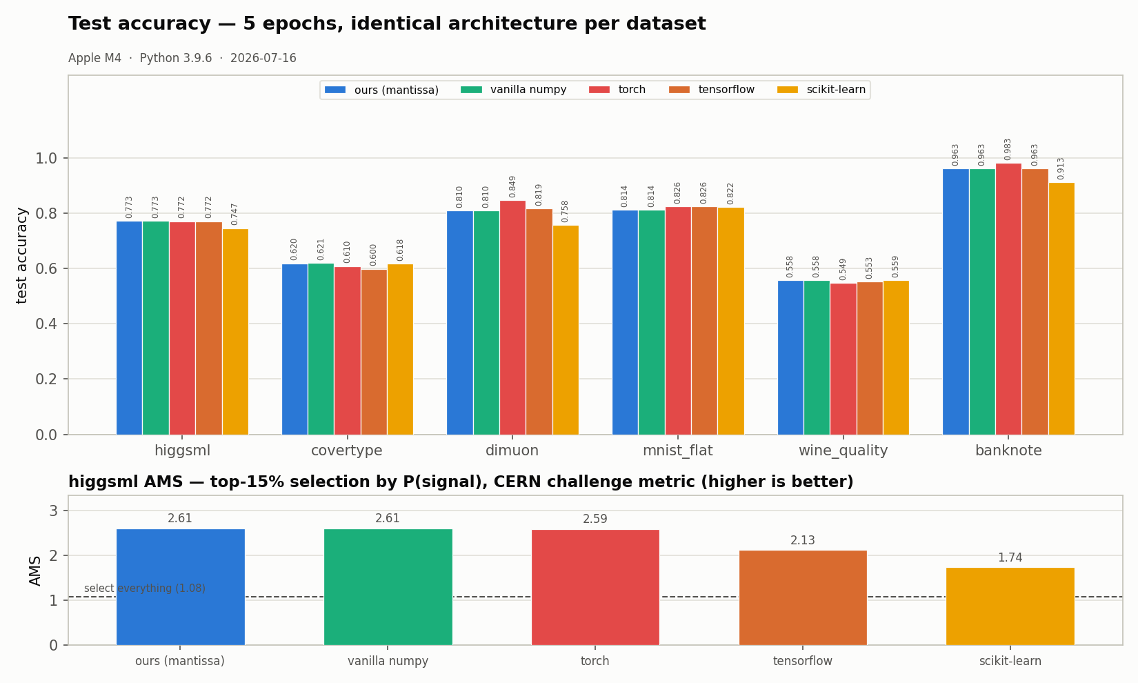
Every contender clears the select-everything baseline (AMS 1.08); selecting nothing scores 0 by construction. ours and its numpy oracle are numerically identical (same math, two backends); torch is within noise; the gap to tensorflow and scikit-learn on AMS tracks their slightly lower accuracy and probability calibration feeding the same cut. This is a teaching-scale reproduction — a 4000-event subset, 5 epochs, no ensemble, momentum or dropout — not a leaderboard pipeline.
All six datasets
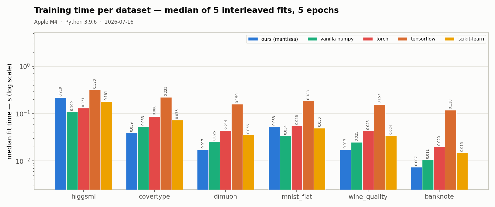
Median fit time over 5 interleaved repeats (s, lower is better) and test
accuracy. sklearn shares an identical parameter count on the four
multiclass sets; on the two binary sets (higgsml, banknote) its single
logistic output unit is last_hidden+1 short of the 2-logit softmax head —
a documented sigmoid-vs-softmax difference, asserted in bench/contenders.py.
| dataset (train/test, classes) | metric | ours | vanilla numpy | torch | tensorflow | scikit-learn |
|---|---|---|---|---|---|---|
| higgsml (4000/2000, 2) | fit s | 0.219 | 0.109 | 0.131 | 0.320 | 0.181 |
| acc | 0.773 | 0.773 | 0.772 | 0.772 | 0.747 | |
| covertype (4000/2000, 7) | fit s | 0.039 | 0.053 | 0.088 | 0.223 | 0.073 |
| acc | 0.620 | 0.621 | 0.610 | 0.600 | 0.618 | |
| dimuon (2000/1000, 3) | fit s | 0.017 | 0.025 | 0.044 | 0.159 | 0.036 |
| acc | 0.810 | 0.810 | 0.849 | 0.819 | 0.758 | |
| mnist_flat (2000/1000, 10) | fit s | 0.053 | 0.034 | 0.056 | 0.188 | 0.050 |
| acc | 0.814 | 0.814 | 0.826 | 0.826 | 0.822 | |
| wine_quality (2000/957, 3) | fit s | 0.017 | 0.025 | 0.043 | 0.157 | 0.034 |
| acc | 0.558 | 0.558 | 0.549 | 0.553 | 0.559 | |
| banknote (916/300, 2) | fit s | 0.007 | 0.011 | 0.020 | 0.118 | 0.015 |
| acc | 0.963 | 0.963 | 0.983 | 0.963 | 0.913 |
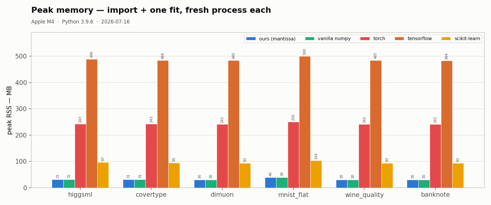
Peak RSS is essentially flat per framework across datasets: ours and the
numpy backend ~30–40 MB, scikit-learn ~93–104 MB, torch ~242–250 MB,
tensorflow ~484–500 MB (import + one fit, fresh process). The raw per-pair
numbers and every timing sample live in bench/results/speed.json.
What the numbers say (honestly)
- Memory is the clean win. ours carries the C engine's whole training footprint in ~30 MB — an order of magnitude under scikit-learn, ~8× under torch, ~16× under tensorflow. That gap is the point of a small dependency.
- Small dense shapes go to ours. On the four
tabular_mlpsets (64→32 hidden) ours has the fastest fit — the C engine's Dense/SGD kernels beat everyone once the per-op dispatch is amortized over enough tiny batches. - Big shapes go to fused BLAS. On the two largest layers — higgsml's
300-wide stack and mnist_flat's 784-wide input — ours loses to its own
numpy backend (0.219 vs 0.109 s; 0.053 vs 0.034 s). At those widths
numpy's fused Accelerate
gemmis already near-optimal, and the mantissa Session's per-primitive Python/ctypes dispatch is pure overhead on top of a comparable kernel. An honest loss, and a clear place to optimize. - torch tracks ours closely; tensorflow's eager
keras.fitcarries the most per-step Python overhead (and itspredict()is 17–33 ms of graph plumbing versus sub-millisecond for everyone else — a batch-inference tax, not a training one). - scikit-learn earns its place. Its Cython SGD is genuinely quick — competitive with ours on the small sets — which is why it is a full contender here. It trails only on the binary sets (its single logistic head and its own initializer, at a 5-epoch budget) and on AMS.
- Accuracy is a near-tie across the softmax family (ours ≡ numpy exactly); differences are a point or two of subset/init noise, not a framework verdict.
Fairness caveats
Identical architecture, epochs, batch size, learning rate and seed for every
contender where the API allows; He-normal / Glorot-uniform init matched
across ours, torch and tensorflow. scikit-learn draws its own init (no
hook to match) and, on binary problems, uses one logistic output unit rather
than a 2-logit softmax — both recorded, not papered over. keras is built and
compiled outside the timed region, and every contender gets one untimed
warm-up fit, so one-time graph tracing / kernel-dispatch caching is excluded
the same way imports are. CPU only; thread knobs left at each framework's
default and recorded, not equalized (mantissa 10, torch 4, tensorflow
runtime-chosen). Two subset budgets were clamped because the frozen protocol
asked for more than a minority class holds: banknote 1000/300 → 916/300
and wine_quality 2000/1000 → 2000/957 (largest feasible equal-stratified
size, seed unchanged; both requested and actual sizes are in the JSON). Peak
RSS loads a cached standardized subset, not the 818k-row higgsml CSV, so the
column is the framework's footprint rather than a 386 MB np.loadtxt
transient shared by all.
Environment
Apple M4 · Python 3.9.6 · numpy 2.0.2 · mantissa ≥0.2.1 · torch 2.8.0 · tensorflow 2.20.0 / keras 3.10.0 · scikit-learn 1.6.1 · 2026-07-16. Total timed region: 47 s (medians over 5 interleaved repeats × 5 contenders × 6 datasets, plus 30 fresh-process RSS measurements).
Reproduce
python -m mantissa_mlp.datasets download all   # fetch any missing datasets
python -m bench.contenders                      # structural parity check
python -m bench.speed                           # timed run (holds /tmp/mantissa-bench.lock)
python -m bench.plots                           # regenerate assets/*.png
Methodology
Identical architectures, subsets, epochs, batch size, learning rate and seeds for every contender; timings are medians over interleaved repeats on one machine, library versions recorded in the results JSON. Peak RSS is measured per contender in a fresh subprocess because that is what a user pays. Measure, don't assume.
License
MIT — © Tekin Ertekin. Base package: mantissa-cnn; engine: mantissa — same author, MIT. The CERN figures and datasets carry their own licenses, credited above: the two Open Data records are CC0, the three photographs CC BY-SA 3.0, the concept diagram CC BY-SA 4.0.
1 maintainer

Metadata
1 maintainer
Release files for mantissa-mlp 0.1.2
For a detailed explanation of source distributions (sdists) and built distributions (wheels), please see the package formats documentation.
Source distribution (sdist)
| File | Size | Uploaded | Provenance | |
|---|---|---|---|---|
| mantissa_mlp-0.1.2.tar.gz | 46.7 kB | With provenance | Details |
Built distribution (wheel)
| File | Interpreter | ABI | Platform | Reset |
|---|---|---|---|---|
| mantissa_mlp-0.1.2-py3-none-any.whl | Python 3 | none | any | Details |
Total release size: 77.7 kB
Release files / mantissa_mlp-0.1.2.tar.gz
| Download URL | mantissa_mlp-0.1.2.tar.gz |
|---|---|
| Size | 46.7 kB |
| Tags | Source |
|
SHA-256 checksum How to use checksums |
8611012ea7c4db518d57f4f337f2003a3cac1ff2ac543cf1a0df2726d1fc55f2
|
|
BLAKE2b-256 checksum How to use checksums |
286dded992575713def5162c069afa8c817a9ef25ac62b8997361a21ed6fa8c0
|
| Upload date | |
|
Uploaded using Trusted Publishing? What is trusted publishing? |
Yes |
| Uploaded via |
twine/6.1.0 CPython/3.13.12
|
Provenance
Provenance describes where a file came from. On PyPI, provenance is shared via attestations, which provide a verifiable record of the build or publishing details. View details, limitations and caveats.


PyPI Publish Attestation
PyPI verified that this artifact, at this checksum, originated from the publisher listed below.
Signed by GitHub Actions, verified by PyPI on Jul 19, 2026.
Transparency logRelease files / mantissa_mlp-0.1.2-py3-none-any.whl
| Download URL | mantissa_mlp-0.1.2-py3-none-any.whl |
|---|---|
| Size | 31.0 kB |
| Tags | Python 3 |
|
SHA-256 checksum How to use checksums |
2a308115a4f4508db9517680d1ce1f16a9dc0684727e71f60d834f924b0e538a
|
|
BLAKE2b-256 checksum How to use checksums |
791ab214d9b7e0b1452f74dbaef9ad8c87df7f0acbd918c261f8687bd4674647
|
| Upload date | |
|
Uploaded using Trusted Publishing? What is trusted publishing? |
Yes |
| Uploaded via |
twine/6.1.0 CPython/3.13.12
|
Provenance
Provenance describes where a file came from. On PyPI, provenance is shared via attestations, which provide a verifiable record of the build or publishing details. View details, limitations and caveats.
PyPI Publish Attestation
PyPI verified that this artifact, at this checksum, originated from the publisher listed below.
Signed by GitHub Actions, verified by PyPI on Jul 19, 2026.
Transparency logSecurity for mantissa-mlp 0.1.2
Provenance
Provenance describes where a file came from. On PyPI, provenance is shared via attestations, which provide a verifiable record of the build or publishing details. View details, limitations and caveats.
Full provenance
All 2 files in this release have been uploaded with provenance metadata.
Attestation for mantissa_mlp-0.1.2.tar.gz
PyPI Publish Attestation
PyPI verified that this artifact, at this checksum, originated from the publisher listed below.
Signed by GitHub Actions, verified by PyPI on Jul 19, 2026.
Transparency logA note on package security
PyPI is a repository for distributing packages, not a service for auditing them. While third-party security researchers and our staff do their best to detect and remove malicious packages, PyPI cannot guarantee the quality, security or suitability of any given package.
To learn more about protecting yourself from malicious actors, visit our package security documentation.

















