
mantissa-perceptron



Perceptron classifier in Python, powered by the mantissa C engine. Rosenblatt
- ADALINE rules, classic UCI datasets, honest benchmarks vs scikit-learn and TensorFlow — faster fit than scikit-learn on every dataset, 3.6× leaner RAM, ~4× faster batch predict.
Rosenblatt's perceptron, with a C engine.
A minimal binary classifier (fit / predict / score) whose compute runs
in mantissa — a fast, memory-lean
neural-network core in C. The Python layer is thin on purpose: the forward
pass, and under the delta rule the entire training step, happen in C on
zero-copy float32 buffers.
Two classic rules, both honest about what they are:
rule="perceptron"— Rosenblatt (1958), mistake-driven; converges in finitely many mistakes on linearly separable data (Novikoff, 1962).rule="delta"— Widrow-Hoff LMS / ADALINE (1960); each step is a singletk_train_step_f32call into the engine. The one to use when the data is not separable.
Both rules are unpacked in plain language (with the papers) in New to perceptrons?
Minimal on purpose: binary only, dense float32, no multiclass, no sparse. sklearn-like interface, not sklearn-compatible.
Install
pip install mantissa-perceptron
This pulls in the engine (mantissa-core) automatically.
From a checkout (works today, no PyPI needed): clone this repo next to
mantissa, build the engine
(make dist there), then pip install -e . here — the package finds the
sibling checkout automatically.
Quickstart
from mantissa_perceptron import Perceptron, datasets

X, y = datasets.load("banknote")            # prints the curl command if missing
Xtr, Xte, ytr, yte = datasets.split(X, y)   # seeded, stratified, standardized
clf = Perceptron().fit(Xtr, ytr)
print(clf.score(Xte, yte))
New to perceptrons? The four ideas in this package
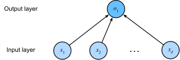
The single neuron. A perceptron is one artificial neuron: it multiplies
each input feature by a learned weight, adds them up with a bias term, and
answers with the sign — y = step(w·x + b). Geometrically the weights are a
learned direction in feature space and the bias slides the decision line
along it: everything on one side of the hyperplane w·x + b = 0 is class 1,
everything on the other side is class 0. The unit dates to the
McCulloch & Pitts (1943) threshold neuron ("A Logical Calculus of the Ideas
Immanent in Nervous Activity", Bulletin of Mathematical Biophysics 5);
what Rosenblatt added was a way to learn the weights from examples
(Rosenblatt, 1958, "The Perceptron: A Probabilistic Model for Information
Storage and Organization in the Brain", Psychological Review 65(6)):
The mistake-driven rule (rule="perceptron"). Rosenblatt's rule only
acts when the neuron is wrong: predict, and on a mistake nudge the weights
toward the missed sample — w += lr·t·x with targets t ∈ {−1, +1} (a
correct answer changes nothing). The surprise is that this converges: if any
hyperplane separates the two classes with margin γ, the rule finds one after
at most (R/γ)² mistakes — a finite bound that does not even depend on the
number of samples (Novikoff, 1962, "On Convergence Proofs on Perceptrons",
Proc. Symposium on the Mathematical Theory of Automata). That is why the
iris row in the accuracy table below converges in 3 epochs, exactly as the
theorem promises.
The delta / LMS rule (rule="delta"). ADALINE's alternative (Widrow &
Hoff, 1960, "Adaptive Switching Circuits", IRE WESCON Convention Record)
updates on every sample, not just mistakes: it runs gradient descent on
the squared error of the linear output w·x + b before the step is
applied — w += lr·(t − w·x − b)·x. Because the objective is a smooth bowl
rather than a count of mistakes, it settles to the least-squares boundary
even when no perfect separator exists — the case where the mistake-driven
rule oscillates forever. That is the rule to reach for on non-separable
data, and it is why delta wins on pima below.
The famous limit. A single neuron can only draw one line, so it cannot represent XOR — no line puts (0,0) and (1,1) on one side and (0,1) and (1,0) on the other. Minsky & Papert made the limits precise in Perceptrons (MIT Press, 1969), and the fix is a hidden layer between input and output — mantissa (the engine under this package) trains XOR with exactly that, and mantissa-cnn keeps stacking from there:
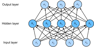
Concept diagrams by Zhang, Lipton, Li & Smola, Dive into Deep Learning, licensed CC BY-SA 4.0 — redistributed here with attribution, unmodified. The same source and license as the concept diagrams in the sister repo mantissa-cnn.
Datasets
Five small classics (UCI + the standard Pima mirror). Nothing downloads
implicitly — data/ is gitignored and library code never touches the
network. Fetch explicitly:
python -m mantissa_perceptron fetch all     # or a single name
python -m mantissa_perceptron list
| name | n | d | task |
|---|---|---|---|
| iris | 100 | 4 | setosa vs versicolor (linearly separable) |
| banknote | 1372 | 4 | genuine vs forged banknotes |
| breast_cancer | 569 | 30 | WDBC malignant vs benign |
| sonar | 208 | 60 | mine vs rock |
| pima | 768 | 8 | diabetes onset |
One real held-out test sample from each, with the trained model's answer
under it (rule="perceptron", the fixed protocol: 75/25 stratified split
seed 42, standardized features, 100 epochs, seed 0; feature values shown
raw, pre-standardization, so they stay human-readable). Correctly-classified
examples — the measured accuracy per dataset and rule is in
Accuracy:
| iris | banknote | breast_cancer | sonar | pima |
|---|---|---|---|---|
| petal 1.7 cm, sepal 5.4 cm | wavelet var 3.62, skew 8.67 | mean radius 18.25, mean area 1040 | 60 sonar bands, peak 1.00@28 | glucose 85, BMI 26.6, age 31 |
| → setosa ✓ | → genuine ✓ | → malignant ✓ | → rock ✓ | → no diabetes ✓ |
Results
Accuracy
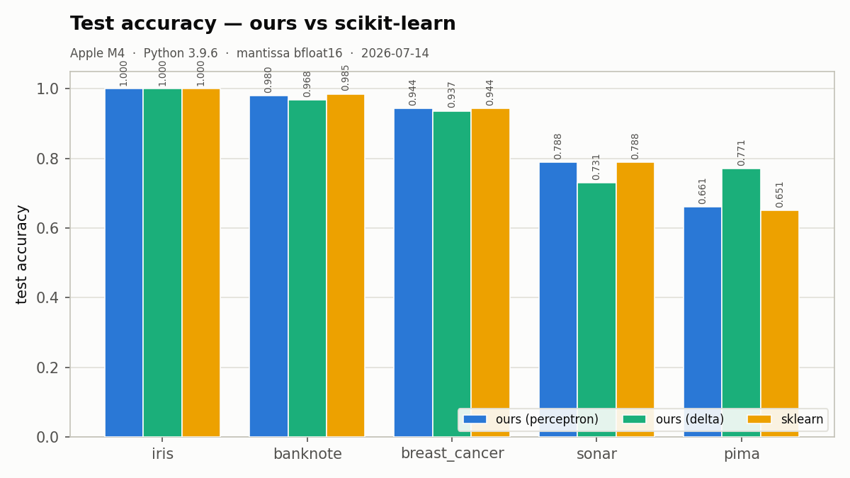
Test accuracy on the held-out 25% (stratified split, seed 42, features
standardized on train statistics only), 100 epochs. The perceptron rule
uses lr=1.0 (the boundary is lr-invariant at zero-init); the delta
(ADALINE) rule's lr is tuned per dataset on the train set only over
{0.001, 0.003, 0.01, 0.03}. Numbers as measured by python -m bench.accuracy.
| dataset | n | d | rule | lr | train acc | test acc | epochs run | converged |
|---|---|---|---|---|---|---|---|---|
| iris | 100 | 4 | perceptron | 1 | 1.000 | 1.000 | 3 | yes |
| iris | 100 | 4 | delta | 0.001 | 1.000 | 1.000 | 1 | yes |
| banknote | 1372 | 4 | perceptron | 1 | 0.991 | 0.980 | 100 | no |
| banknote | 1372 | 4 | delta | 0.001 | 0.980 | 0.968 | 100 | no |
| breast_cancer | 569 | 30 | perceptron | 1 | 0.995 | 0.944 | 100 | no |
| breast_cancer | 569 | 30 | delta | 0.001 | 0.970 | 0.937 | 100 | no |
| sonar | 208 | 60 | perceptron | 1 | 0.929 | 0.788 | 100 | no |
| sonar | 208 | 60 | delta | 0.001 | 0.910 | 0.731 | 100 | no |
| pima | 768 | 8 | perceptron | 1 | 0.674 | 0.661 | 100 | no |
| pima | 768 | 8 | delta | 0.001 | 0.780 | 0.771 | 100 | no |
iris is linearly separable, so the perceptron converges to a perfect boundary (Novikoff). banknote and breast_cancer are nearly separable. On the non-separable sets the honest picture shows: sonar (60 features, 208 samples) overfits — high train, weak test; pima is genuinely hard for a linear model, and there the delta rule's smoother LMS objective beats the oscillating mistake-driven rule on both train and test.
Speed and memory vs famous implementations
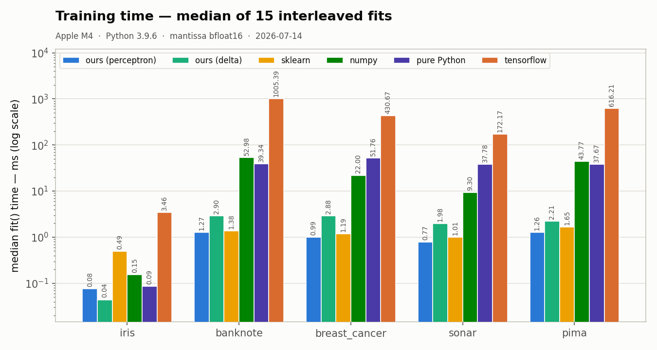
On the largest dataset (banknote, 1372×4, 100-epoch cap, 15 interleaved repeats, medians):
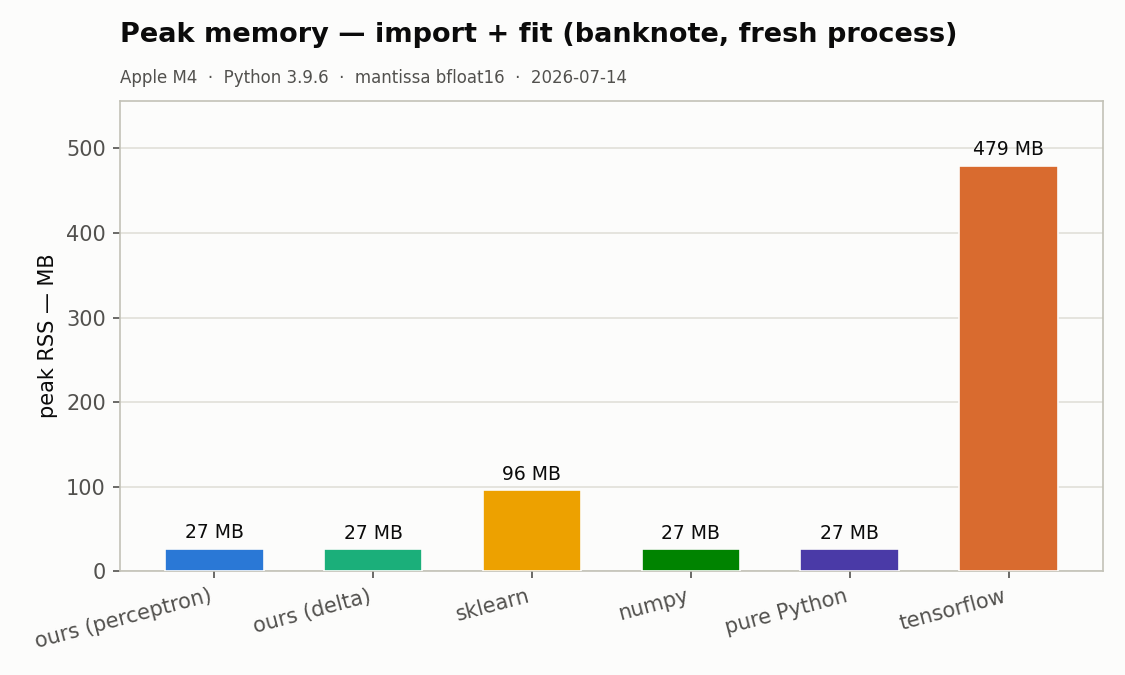
| contender | fit (ms) ↓ | predict (ms) ↓ | peak RSS (MB) ↓ |
|---|---|---|---|
| ours (perceptron) | 1.27 | 0.013 | 26.8 |
| ours (delta) | 2.90 | 0.010 | 26.7 |
| scikit-learn | 1.38 | 0.050 | 96.4 |
| numpy (hand-rolled) | 52.98 | 0.006 | 26.7 |
| pure Python | 39.34 | 0.091 | 26.7 |
| TensorFlow | 1005.39 | 0.051 | 479.4 |
torch omitted — not importable in this environment; the harness includes it automatically when it is.
The story of this table is the three engine releases it forced. The first
run measured our fits at 661 ms (delta) and 535 ms (Rosenblatt) — every
training sample paid a Python→C crossing. Each finding went upstream
(docs/LEARNINGS.md): mantissa v0.1.11 moved the delta
epoch into one C call (661 → 4.4 ms), the dataset-epoch primitives moved the
Rosenblatt rule and the shuffle order in as well, and v0.1.14 attacked what
profiling showed was left — the crossings themselves:
- Rosenblatt: 535 → 1.81 → 1.27 ms (420×) — one
tk_perceptron_epoch_f32call per epoch, mistake count included; thentk.trainer()(v0.1.14) binds the W/X/targets/bias pointers once per fit instead of re-deriving them every epoch (measured: the old per-epoch call spent ~7 µs of its 9.8 µs on ctypes pointer conversion, only ~3 µs in C). Now faster than scikit-learn's Cython SGD on all five datasets, with honest early stopping (we stop at zero training mistakes; sklearn withtol=Nonenever does — on separable data our fit is a few epochs, not 100). - Delta: 661 → 3.68 → 2.90 ms — ordered epochs (the shuffle permutation crosses as an int32 index array; no per-epoch row copies), the same pre-bound pointers, plus one post-epoch convergence pass, kept deliberately: LMS updates on every sample, so only a post-epoch count certifies the final weights (an in-epoch count was measured faster but rejected on exactly that semantic). The residual gap to sklearn is the rule, not the plumbing: LMS writes the weights on every sample where the mistake-driven rules write only on errors.
- Memory: 26.8 MB vs scikit-learn's 96.4 — 3.6× leaner; TensorFlow's import alone peaks at 479 MB, 18× ours.
- Batch predict: 0.013 ms — ~4× faster than scikit-learn (one threaded C call into a caller buffer).
- Accuracy: unchanged and at parity with scikit-learn — the v0.1.14
trainer is pinned bit-identical to the previous path (same C entry points,
same RNG stream), and the
bench/accuracy.pyre-run under mantissa v0.2.3 confirms byte-identical results. - TensorFlow, honestly measured: the same mistake-driven rule with the
whole epoch compiled as one
@tf.functiongraph (tracing excluded, like imports). Sequential per-sample updates are simply not TF's shape — eachtf.while_loopstep dispatches kernels — so it lands ~800× behind the C epoch. Its batch predict (0.051 ms) is competitive; the gap is the training loop, not the framework's math.
Fairness caveats.
- scikit-learn's
Perceptronis Cython SGD doing strictly more bookkeeping per epoch than the naive rule; our remaining per-epoch overhead is one ctypes crossing plus the Python-siderng.permutation(6.4 µs at n=1030 — measured faster than every batching alternative we tried). - We set
tol=Noneon scikit-learn to disable its early stopping and equalize the 100-epoch budget; our early stop fires only at zero training mistakes. numpy/pure Pythonimplement the same mistake-driven rule in-process and are the honest baseline for what the old per-sample FFI loop was costing.- TensorFlow runs the identical rule and epoch/shuffle protocol; only graph tracing (a one-time compile) is excluded from fit timing. Eager TF was ~100× slower still and would have benchmarked the interpreter, not TF.
Environment. Apple M4 · Python 3.9.6 · numpy 2.0.2 · scikit-learn 1.6.1 ·
TensorFlow 2.20.0 · mantissa 0.2.3 dtype bfloat16 · threads default(10) ·
2026-07-14. Full raw samples and versions in bench/results/speed.json
(regenerable, gitignored). Re-measured for the v0.2.3 engine (an audit
release that does not touch this package's code path): every median
reproduced within ±3% of the previous run and no ratio moved — day-to-day
machine noise the interleaved protocol is designed to absorb.
Methodology
Fixed protocol: stratified 75/25 split (seed 42), features standardized on
train statistics only, epochs capped identically for every contender.
Timings are medians over interleaved repeats on one machine (library
versions and CPU recorded in bench/results/speed.json); peak RSS is
measured per contender in a fresh subprocess, import cost included, because
that is what a user pays. Measure, don't assume.
License
MIT — © Tekin Ertekin. Engine: mantissa, same author, MIT.
1 maintainer

Metadata
1 maintainer
Release files for mantissa-perceptron 0.1.0
For a detailed explanation of source distributions (sdists) and built distributions (wheels), please see the package formats documentation.
Source distribution (sdist)
| File | Size | Uploaded | Provenance | |
|---|---|---|---|---|
| mantissa_perceptron-0.1.0.tar.gz | 23.5 kB | With provenance | Details |
Built distribution (wheel)
| File | Interpreter | ABI | Platform | Reset |
|---|---|---|---|---|
| mantissa_perceptron-0.1.0-py3-none-any.whl | Python 3 | none | any | Details |
Total release size: 41.5 kB
Release files / mantissa_perceptron-0.1.0.tar.gz
| Download URL | mantissa_perceptron-0.1.0.tar.gz |
|---|---|
| Size | 23.5 kB |
| Tags | Source |
|
SHA-256 checksum How to use checksums |
58a5b93cfdc00ff2a506671171786f742fa0a530e82c1c9e18ebeea3f2924f00
|
|
BLAKE2b-256 checksum How to use checksums |
c6e1a70a78c7825f31a8331158ffc490df98f92bdde7683a173b42767d3d9a89
|
| Upload date | |
|
Uploaded using Trusted Publishing? What is trusted publishing? |
Yes |
| Uploaded via |
twine/6.1.0 CPython/3.13.12
|
Provenance
Provenance describes where a file came from. On PyPI, provenance is shared via attestations, which provide a verifiable record of the build or publishing details. View details, limitations and caveats.


PyPI Publish Attestation
PyPI verified that this artifact, at this checksum, originated from the publisher listed below.
Signed by GitHub Actions, verified by PyPI on Jul 18, 2026.
Transparency logRelease files / mantissa_perceptron-0.1.0-py3-none-any.whl
| Download URL | mantissa_perceptron-0.1.0-py3-none-any.whl |
|---|---|
| Size | 18.0 kB |
| Tags | Python 3 |
|
SHA-256 checksum How to use checksums |
b53b9ab8694b64bfdb28abc0f3657a9f6d82a6e32530cb172b8d666260029f71
|
|
BLAKE2b-256 checksum How to use checksums |
832dcf6f3604612d6e4d20f4b922bd30c81eaf1e5f4c968d4cf7f97dfc8599b4
|
| Upload date | |
|
Uploaded using Trusted Publishing? What is trusted publishing? |
Yes |
| Uploaded via |
twine/6.1.0 CPython/3.13.12
|
Provenance
Provenance describes where a file came from. On PyPI, provenance is shared via attestations, which provide a verifiable record of the build or publishing details. View details, limitations and caveats.
PyPI Publish Attestation
PyPI verified that this artifact, at this checksum, originated from the publisher listed below.
Signed by GitHub Actions, verified by PyPI on Jul 18, 2026.
Transparency logSecurity for mantissa-perceptron 0.1.0
Provenance
Provenance describes where a file came from. On PyPI, provenance is shared via attestations, which provide a verifiable record of the build or publishing details. View details, limitations and caveats.
Full provenance
All 2 files in this release have been uploaded with provenance metadata.
Attestation for mantissa_perceptron-0.1.0.tar.gz
PyPI Publish Attestation
PyPI verified that this artifact, at this checksum, originated from the publisher listed below.
Signed by GitHub Actions, verified by PyPI on Jul 18, 2026.
Transparency logA note on package security
PyPI is a repository for distributing packages, not a service for auditing them. While third-party security researchers and our staff do their best to detect and remove malicious packages, PyPI cannot guarantee the quality, security or suitability of any given package.
To learn more about protecting yourself from malicious actors, visit our package security documentation.













