

Segmentation and other dense-prediction models for PyTorch, built from
timm encoders.
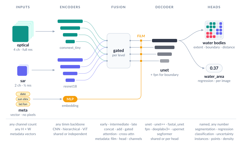
Any number of bands, several inputs at different resolutions, metadata, and many outputs in one model.
Model builder: design a model in your browser and copy the code.
Documentation · PyPI
Status: alpha. Before 1.0 the API may change between minor versions; every change is listed in
CHANGELOG.md.
Install
Python ≥ 3.11, PyTorch ≥ 2.10:
pip install manyseg
# or
uv add manyseg
Optional extras: [quant] (int8 quantisation), [onnx] (ONNX export), [instances]
(instance post-processing), [vectors] (polygons, road graphs and points as GIS layers), e.g.
pip install "manyseg[vectors]" or uv add "manyseg[vectors]".
Quick start
import torch
from manyseg import create_model

model = create_model(backbone="convnext_tiny", in_channels=4, num_classes=3)  # U-Net by default
logits = model(torch.randn(2, 4, 257, 301))   # (2, 3, 257, 301): any size, odd or non-square
print(model.describe())                       # what was built, stage by stage
backbone is a timm model name: ResNet, EfficientNet, ConvNeXt, Swin, PVTv2, ViT, DINOv2 and
most other timm families that expose multi-scale features. 46 models are tested
(compatibility table); a few only accept inputs up to a fixed
size. Pretrained weights are the default (pretrained=True): timm downloads them on first use
and they are adapted to your band count. Pass pretrained=False to skip the download.
The model does not normalise its input: scale or standardise your bands as you would for any
timm model. Each pretrained weights saw RGB as (x - mean) / std with its own statistics:
ImageNet's for most; of the tested backbones, 0.5 / 0.5 for ViT AugReg, SigLIP,
tf_efficientnetv2_s and coatnet_0_rw_224, and CLIP's for EVA-02. describe() and
manyseg.weights.attribution(model) show the values. With num_classes= the output is one
tensor of raw logits; with heads= it is a dict of raw logits keyed by head name.
Model builder
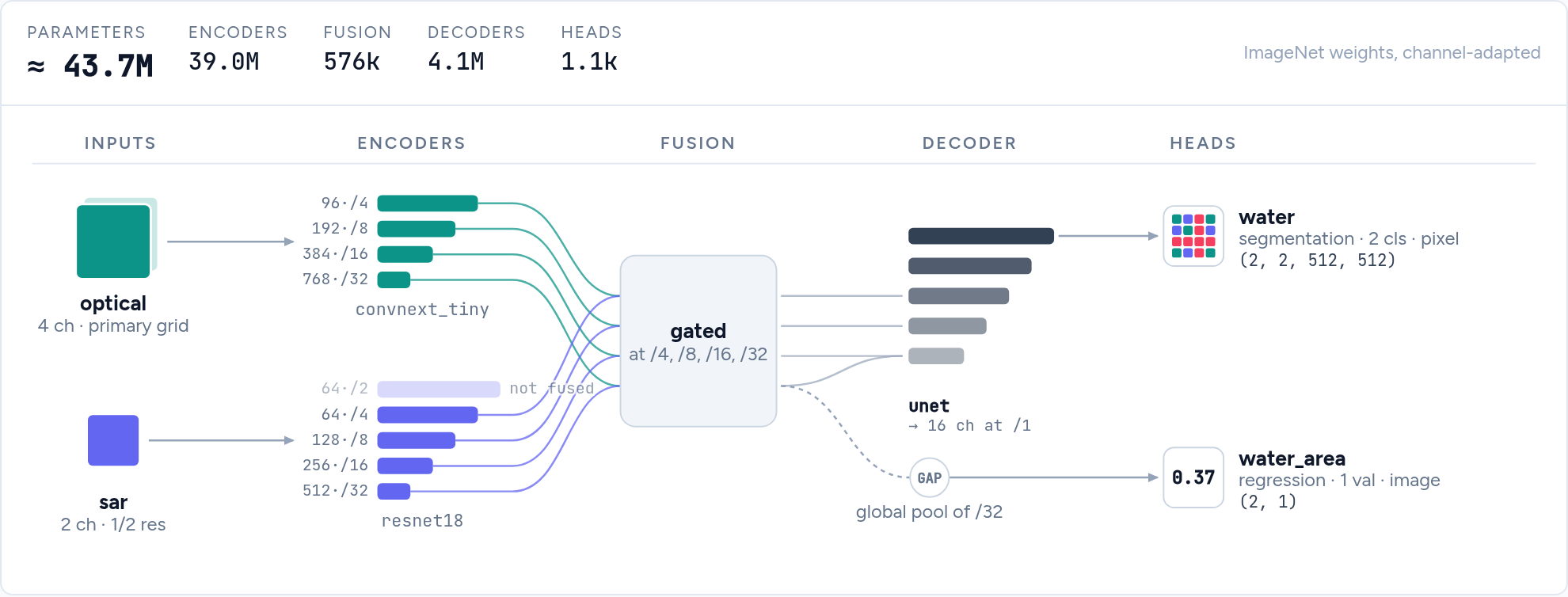
Not sure how to combine inputs, fusion and heads? The model builder draws the
model as you pick options and writes the create_model call, refusing combinations ManySeg would
reject. It runs in the browser; offline, open docs/builder/index.html from a clone of this
repository.
Common tasks
Multispectral imagery. Set in_channels (e.g. 13 for Sentinel-2). The pretrained RGB stem
is adapted automatically. For extra channels that are not image bands (validity masks, quality
flags), use channel_adapter="rgb_plus_zero". If bands can be missing at inference, fill them
the way you did in training and drop bands at random while training
(missing bands).
Several inputs, possibly at different resolutions, e.g. optical + radar. If your bands share a grid, stack them into one input first: that matched separate encoders on Sen1Floods11 (E005). Separate encoders are for inputs at different resolutions, or for when stacking falls short:
model = create_model(
    inputs={
        "optical": {"in_channels": 4, "backbone": "convnext_tiny"},
        "sar": {"in_channels": 2, "backbone": "resnet18", "alignment": "same_extent"},  # half res OK
    },
    fusion={"type": "intermediate", "op": "concat"},
    num_classes=2,
)
out = model({"optical": optical, "sar": sar})
Several outputs. Name your heads; the model returns a dict:
model = create_model(
    backbone="resnet50", in_channels=4,
    heads={
        "landcover": {"type": "segmentation", "out_channels": 8},
        "height":    {"type": "regression", "out_channels": 1},                  # per pixel
        "flooded":   {"type": "classification", "out_channels": 2, "scope": "image"},
    },
)
A pixel head is one 3×3 conv, as in SMP. For a wider one, give it hidden layers, e.g.
"hidden": [64, 32, 16], "dilation": [8, 16, 32] for a receptive field that matches large
objects. Any head can also get its own decoder ("decoder": "unet"), or be your own class
registered with manyseg.heads.HEADS.register("name").
Training. A model is a plain nn.Module, so any trainer works. There are examples for
fastai, a plain PyTorch loop,
Lightning, Accelerate and
TorchGeo (its segmentation task with a ManySeg model), all tested
in CI. With several heads, a loss and metrics read the dict (out["landcover"]), or
manyseg.utils.concat_heads(model, ["landcover", "height"]) wraps the model so it returns one
concatenated tensor, for code that wants one. manyseg.losses has the losses our benchmarks
train with (Dice + BCE,
multi-class Dice, masked regression, CenterNet heatmap focal loss) as plain functions, and
multi_head_loss sums a weighted loss per head of the output dict.
A model with metadata inputs takes a dict, so a loop that passes one tensor needs a small
wrapper of your own that builds it. Save the model inside, not the wrapper
(manyseg.save(wrapper.model, ...)), and wrap manyseg.load(path) again after loading.
Image classification or regression. Use only image heads: no decoder is built, and the model is a classifier that still accepts several inputs, metadata and extra heads.
model = create_model(backbone="resnet50", in_channels=12, heads={
    "labels": {"type": "classification", "out_channels": 19, "scope": "image"}})
If you also have pixel labels, training with an extra segmentation head can improve the
classifier. Drop it before deployment with model.select_heads(["labels"]) (in place: the
model keeps only that head and its output stays a dict).
Metadata (acquisition date, sun angle, location, sensor) as extra inputs:
inputs = {
    "image": {"in_channels": 4},
    "meta": {"kind": "vector", "fields": {"doy": {"type": "cyclic", "period": 365.25},
                                          "latlon": {"type": "coords"}}},  # degrees, lat first
}
model = create_model(inputs=inputs, num_classes=2)
meta = model.pack_metadata("meta", {"doy": torch.tensor([45.0, float("nan")]),  # NaN = missing
                                    "latlon": torch.tensor([[-31.9, 115.9], [-33.9, 18.4]])})
out = model({"image": torch.randn(2, 4, 128, 128), "meta": meta})
The model takes the packed (B, N) tensor; pack_metadata builds it from per-field values,
and NaN marks a missing value. In our tests metadata rarely helped, so compare against a model
without it on your data.
Time series. One encoder runs on every date and the dates are combined per level (mean,
max, attention, ...); pass (B, T, C, H, W) plus optional "s2_mask" / "s2_dates":
model = create_model(inputs={"s2": {"kind": "timeseries", "in_channels": 10}}, num_classes=20)
out = model({"s2": torch.randn(2, 6, 10, 128, 128)})        # any number of dates
Change detection. Two dates through one shared (Siamese) encoder, a difference fusion, and optionally a land-cover head per date (semantic change):
model = create_model(
    inputs={"t1": {"in_channels": 3},
            "t2": {"in_channels": 3, "backbone": "shared:t1", "share_norm": True}},
    fusion={"type": "intermediate", "op": "diff"},
    heads={"change": {"type": "segmentation", "out_channels": 2},
           "lc1": {"type": "segmentation", "out_channels": 7, "input": "t1"},
           "lc2": {"type": "segmentation", "out_channels": 7, "input": "t2", "share": "lc1"}},
)
Overlapping classes (e.g. cloud and shadow): one segmentation head with a channel per class, a sigmoid per channel and BCE loss.
Embeddings. model.features(x) returns the encoder pyramid; model.embed(x, pool="mean") gives vectors for retrieval, clustering or probing.
Remote-sensing pretrained weights. create_model(backbone="resnet50", pretrained="ssl4eo_s2_dino", in_channels=13, ...) loads SSL4EO-S12 weights
(Sentinel-2 MoCo: ResNet-18/50, ViT-S/16; DINO: ResNet-50, ViT-S/16; Sentinel-1 MoCo:
ResNet-50) or SatlasPretrain Sentinel-2 weights (ResNet-50/152); manyseg.weights.WEIGHTS lists the band order and normalisation each
expects. Fed their own pretraining normalisation, SSL4EO DINO weights beat the ImageNet
baseline on all three Sentinel-2 datasets we tested (ResNet-50, full fine-tuning; E024).
The weights are CC BY 4.0 / ODC-BY and need attribution, also once fine-tuned: saved models
record each pretrained backbone's licence and citation, and describe() lists them.
Objects and counts. manyseg.instances (touching fields, crowns, buildings) and
manyseg.points (trees, animals: centres, counts) provide the heads, training targets (from
instance masks, points or YOLO / COCO boxes) and post-processing; the losses, density_loss
among them, are in manyseg.losses (manyseg.points re-exports density_loss). To count, either
find peaks in a centre heatmap (find_peaks, with optional smoothing and a foreground mask)
or sum a density map (density_head, density_loss; count_from_density(density, sigma=)
divides by the target's 2πσ² scale). Which is better depends on the data.
With many small trees per tile, the density head had half the count error of peaks at a fixed
threshold (E011), and about the same once the threshold was calibrated on validation data (test
MAE 19.4 against 20.6; E011b). With a few large plants per drone tile, peak counting was far
better (count MAE 1.0 against 7.5–11 for raw density heads), because a small background bias
summed over every pixel adds up; count peaks for a few large objects. density_head() uses a
softplus output by default: on that drone data its count MAE was 2.9, against 10.1 for the raw
head clamped at 0 and 7.5 summed as is, and on OAM-TCD it was no worse than the raw head (E011c).
Softplus never reaches 0, so every tile sums to a small positive floor (about +1.75 objects per
image, 2.4 on an empty 792 x 792 drone tile); density_head(activation=None) gives the raw
head.
The drone numbers come from one downstream dataset (45 validation images, one seed) and are not
reproduced in this repository. Validate on your data.
Vector outputs (experimental). manyseg.vectors (the [vectors] extra) turns
predictions into GIS layers: building footprints with straight walls, field boundaries,
road graphs with junctions and overpasses, LoD2 roof faces with a plane and 3-D mesh each
(heights from an nDSM input), and points. Each task has a head preset, target encoders that
work in pixel coordinates (to_pixels brings your vector labels there from any CRS), its
training losses and metrics (manyseg.vectors.losses, manyseg.vectors.metrics), and a decoder
tested on one dataset each (docs/api_design.md gives the evidence). One call decodes
a scene of any size: large scenes block by block, with the default 256 px halo. min_halo is
only the smallest halo a decoder accepts and doesn't guarantee the same result as a whole-scene
decode: on noise-like field predictions, halos up to 64 px gave different objects. An instance
reaching much further than the halo can split at a block seam, and for roads the halo must also
cover the skeleton's data-dependent reach (the decoder warns). With ManyPred this happens while
it predicts (needs ManyPred's GitHub main; not yet in a PyPI release).
from manyseg.vectors import Scene, block_decoder, decode_scene

# probs: head name -> the stitched predictions (numpy; sigmoid on the logit heads)
scene = Scene(H, W, transform=src.transform, crs=src.crs)  # the image's grid (rasterio)
records = decode_scene(probs, block_decoder("footprints"), scene=scene)  # 4096 px blocks
records.write("buildings.geojson")  # polygons in the raster's CRS; .gpkg also needs geopandas
Examples 14–18 cover each task from vector labels to GeoJSON; the guide lists the heads, decoders, evidence and limits.
Save and load. manyseg.save stores the weights with the configuration and, as metadata
for inference code, the input normalisation, output activations and class names; manyseg.load
rebuilds the model without downloading anything. activations is required for every
segmentation and classification head (the head type can't tell softmax from sigmoid), and
save raises a ValueError naming the heads without one; regression heads and "softplus"
density heads default to "none". Without normalize, save stores none and warns:
import manyseg

model = manyseg.create_model(in_channels=4, num_classes=2)  # ... then train it
manyseg.save(model, "model.safetensors",
             activations={"logits": "softmax"},             # how each head becomes a prediction
             normalize=[{"type": "scale", "value": 10000}],  # the input scaling you trained with
             classes=["background", "water"])
model = manyseg.load("model.safetensors")
meta = manyseg.read_metadata("model.safetensors")  # the stored normalize / activations / classes
The loaded model still takes the raw-scale input you trained on and returns logits: applying
the stored normalisation and activations is up to the inference code. The default head of a
num_classes= model is named "logits".
Share on the Hugging Face Hub. manyseg.push_to_hub takes save's metadata arguments
(normalize, activations, classes, bands, extra), saves the model as
model.safetensors, uploads it to a model repository (private by default) and writes a model
card listing the inputs, heads and the licences of the pretrained weights (and, for a quantised
model, that loading needs manyseg[quant]). The repository is a plain org/name; a branch goes
in revision=. It has no source=,
so a quantize_pt2e program (a .pt2 file) can't be pushed. load and read_metadata take
Hub names as timm does:
manyseg.push_to_hub(model, "your-org/water", activations={"logits": "softmax"},
                    normalize=[{"type": "scale", "value": 10000}], license="mit",
                    revision="v1")                  # optional: a branch name, created if needed
model = manyseg.load("hf-hub:your-org/water@v1")   # token=... for a private repository
Both use HF_TOKEN or a stored hf auth login when no token= is given. Tags and commits
can be loaded (@<tag>, @<sha>) but not pushed to.
Don't save the whole model with torch.save(model): that pickle refers to ManySeg's internal
module paths, so it breaks when a later version moves or renames a class, and loading it
needs torch.load(weights_only=False), which can run arbitrary code. A manyseg.save file holds
plain data: the create_model arguments, a save-format number and the weights. When the format
changes, older files are migrated on load, and a file from a newer ManySeg fails with both versions
named. A library that keeps its own table of models (architecture names plus weights) should
store one manyseg.save file per model and call manyseg.load; take
manyseg.load(path).state_dict() if it needs a state dict.
Deployment. Models work with torch.compile(dynamic=True), torch.export and ONNX with
dynamic input sizes (a few encoder families only run at a fixed size or cannot export
dynamically; see the compatibility table), and with int8
quantisation (import manyseg.quantize). For fast GPU inference use bf16
autocast plus torch.compile.
manyseg.save and manyseg.load also handle quantised models, with their metadata and
tiling_spec(), so ManyPred can run them from a file (both need manyseg[quant] to load):
from manyseg.quantize import quantize_pt2e, quantize_weights

# spec: the normalisation steps the model was trained with, e.g. [{"type": "scale", "value": 10000}]
# example: one input batch; batches: a few representative batches for calibration
q = quantize_weights(model)                 # CPU or GPU: an nn.Module with int8 weights
manyseg.save(q, "model_int8.safetensors", normalize=spec, activations={"logits": "softmax"})

ep = quantize_pt2e(model, example, batches)  # CPU: static int8
manyseg.save(ep, "model_int8.pt2", source=model, normalize=spec,
             activations={"logits": "softmax"})
program = manyseg.load("model_int8.pt2")     # a callable with tiling_spec(), not an nn.Module
Only load .pt2 files from sources you trust. manyseg.load refuses the ways we know a crafted
file could run code while loading, but that is not a sandbox, and the program runs when called.
Most of these have a runnable script in examples/ that runs on CPU: the numbered
scripts in a few seconds (5–15 s for 09–13, which train two short epochs), the walkthroughs that
train briefly in 10–20 s.
Large images with ManyPred
A ManySeg model predicts a whole image in one forward pass, so memory limits the image size,
and a fixed-size backbone refuses anything larger than its size. For larger scenes use
ManyPred, our tiled inference library: it predicts
overlapping patches in batches, stitches them, skips nodata, and reads and writes GeoTIFFs
larger than memory. It is a separate library so it can run any PyTorch model that returns a
tensor or a dict of tensors; ManySeg does not import it. It is not on PyPI yet, so install it
from GitHub ([geo] adds rasterio for GeoTIFFs):
pip install "manypred[geo] @ git+https://github.com/DPIRD-DMA/ManyPred"
ManyPred reads the model's tiling_spec() (padding multiple, fixed input size, each head's
resolution) and the normalisation and activations stored by manyseg.save, so with a model
saved as in "Save and load" above neither is repeated. The class and band names you saved are in
the spec too, and predict_files writes them into its output files:
import numpy as np
import manyseg
from manypred import predict_array, predict_files
from manypred.geo import RasterioReader

model = manyseg.load("model.safetensors")
scene = np.random.randint(0, 10000, (4, 3000, 3000), dtype=np.uint16)  # raw scale, (C, H, W)
probs = predict_array(model, scene, patch_size=1024, overlap=256)  # (2, 3000, 3000), softmax

def load(path):  # patches are read as needed, so the scene can be larger than memory
    reader = RasterioReader(path)
    return reader, reader.profile  # the profile georeferences the output

# GeoTIFFs in, GeoTIFFs out (predictions/scene_pred.tif); nodata=0 skips zero-filled borders
predict_files(model, ["scene.tif"], load_func=load, output_dir="predictions",
              patch_size=1024, overlap=256, output="argmax", nodata=0)
device defaults to CUDA, then MPS, then the CPU, and dtype to float32; dtype="float16" or
"bfloat16" is faster on GPUs that support it, and rounds the weights and outputs. Overlapping
patches are blended by default (merge="blend", a weighted mean that fades towards each patch
edge). merge="cut" takes each pixel from the patch it is most central in, so nothing is averaged;
it can be set per head (merge={"extent": "cut"}). Use it for road heads decoded into graphs,
and keep blend for maps used as rasters. On City-Scale roads, blending lost junctions where
patches overlapped (junction agreement with a whole-scene pass 0.954, cut 0.971, away from
overlaps 0.972; E050). For roof faces patch size mattered more: agreement 0.945 (blend) or 0.944
(cut) with 512 px patches and 128 px overlap, and 0.979 (blend) or 0.987 (cut) with 1024 px
patches and 256 px overlap, a gain for cut that wasn't the pre-registered comparison (E050b;
both experiments). Cut and blend haven't been compared
on trained field or footprint models.
The vector decoders (Vector outputs above) run on large scenes through manypred.blocks:
postprocess_blocks decodes saved rasters block by block, and
predict_files(..., merge="cut", block_postprocess=BlockPostprocess(...)) decodes while it
predicts (guide). merge and
manypred.blocks are on ManyPred's GitHub main since 2026-11-02, and will be in its first
release.
ManyPred moves a model to its device and dtype in place and sets it to eval mode. So after a
preview during training, call model.train() (and move it back if it was on another device)
before training further. With dtype="float16" or "bfloat16" the weights are also rounded for
good: reload the model or restore your checkpoint before training further or calling
manyseg.save, or run the preview on a copy, or the weights go on, and are saved, in the lower
precision.
Tips from our benchmarks
- Small batches (measured at 2 per GPU): keep the encoder's BatchNorm layers in eval mode during training (frozen running statistics; their weights still train; recipe).
- Memory-bound?
decoder_kwargs={"out_stride": 2}costs no accuracy for the U-Net and saves 11–18% memory.model.set_grad_checkpointing()recomputes encoder activations in the backward pass: same values, −22% memory for +5% step time on the ResNet-34 U-Net, −61% for +18% on ConvNeXt-T (E026). - Batch-1 inference:
torch.compile(model, mode="reduce-overhead")(CUDA graphs, fixed input size) is up to 1.8× faster than the default compile for PVTv2-b0 models (E026). - Water and other per-pixel spectral targets:
decoder_kwargs={"input_cross": True}feeds the raw bands to the last decoder stage. It did not help pet or cloud segmentation. - Mixed precision is safe: bf16, fp16 and int8 weight-only showed no accuracy loss. One exception: on Windows, PyTorch's CPU bfloat16 can crash with an illegal-instruction error on some processors, so use float32 on the CPU there.
- Training speed: the default U-Net trains as fast as SMP's
Uneton the same timm encoder: compiled steps match it, and eager steps are 18–25% faster (bf16, E025).
These come from experiments in experiments/, where negative results are kept
too. Most are pre-registered and multi-seed; the speed and memory figures (E025, E026) are timing
runs without seeds.
What the evidence says
ManySeg has more options than we have evidence for. An option that showed no gain here may still help on your data, and an untested one is simply unknown.
| Option | Result | Evidence |
|---|---|---|
Separate encoders with concat or gated fusion, vs stacking bands |
no demonstrated gain in the tested shared-grid cases; helped across a 25× resolution gap (one dataset) | Shared grid: E005, Sen1Floods11 (late fusion was worse on test); E056, MFNet RGB + thermal, +0.3 mIoU (1 seed, did not clear the screen). Different scales: E059, FLAIR #2 aerial 0.4 m + Sentinel-2 10 m, +2.9 test mIoU over stacking, mostly because stacking the upsampled S2 was 2.3 below aerial alone; the S2 encoder added little over aerial alone, and a monthly time series showed no demonstrated improvement over a median. E061: a wider S2 window (200 or 400 m instead of the 100 m footprint) did not pass its one-seed screen (−0.001 val mIoU for the better arm, 400 m) |
Fusion ops add, attention, cross_attention |
not tested for accuracy | none |
Siamese encoder with diff or concat_diff, for change detection |
helped | E022, OSCD and LEVIR-CD |
| Per-input land-cover heads, for semantic change | helped | E023, SECOND only |
| Splitting Sentinel-2 bands into resolution groups | mixed | helped in E015; not in E016, E017 or E020 |
| Metadata (FiLM, head bias or channels) | helped on two tasks where the vector carries information the pixels don't fully give | No clear gain for date or location (E009, E013, E016, E020). Helped for zoom in metric depth (E055, NYUv2: FiLM −4% AbsRel, beat channels) and latitude in longitude prediction (E058, ~48k SSL4EO-S12 locations: +4.0 to +10.3 points accuracy, though the shuffled control fell 0.0001 outside its bar; E057, a smaller pilot, agrees). In E058 (image heads) the placement mattered: head < FiLM (pooled feature) < channels ≈ FiLM inside the encoder (hand-written, not a ManySeg option), so try channels for image heads. In E060 (pixel heads, E055's task) FiLM inside the encoder showed no demonstrated improvement over ManySeg's FiLM. E062: Sentinel-2 summary statistics as FiLM for FLAIR #2 aerial segmentation did not pass the one-seed screen (+0.004 val mIoU for the best arm) |
| Time-series input, vs stacking dates as channels | mixed | E021: attention won on field delineation, not on crop types; several dates beat one by a wide margin either way |
fastai_unet, vs the default U-Net |
small gain at high cost | E003 Pet +0.4 test mIoU at 4× FLOPs; E006 Sen1Floods11 +1.7 test mIoU at 4–5× latency |
input_cross |
mixed | E012 helped on Sen1Floods11, not Pet; E013 no gain on clouds |
| UPerNet | tied with the U-Net at more cost | E003, Pet only |
| SegFormer head, FPN, DeepLabV3+ | lower accuracy, on Pet | E003 |
| U-Net++ | not tested for accuracy | E025 measured training speed only |
| Boundary + distance heads, for touching objects | helped | E010, AI4Boundaries: doubled panoptic quality against extent alone |
| An auxiliary segmentation head on an image classifier | helped | E020, BigEarthNet only; looks like regularisation |
| SSL4EO DINO weights with their own normalisation | helped | E024, three Sentinel-2 datasets, ResNet-50 |
| ImageNet RGB weights on Sentinel-2, vs random weights | mixed | E063: helped on CloudSEN12+ (+4.2 points) and PASTIS (+1.0), slightly worse on Sen1Floods11 and BigEarthNet; level with 12–252 labelled chips |
| Footprint decoder (corners and walls) | helped on boundary quality, slightly lower detection | E038, WHU aerial only, 2 seeds |
| Field decoder (instance outlines) | chosen over corners and walls | E046 and E052, Fields of The World Netherlands only, 1–2 seeds |
| Road decoder (unified heads) | kept more overpasses, no loss on APLS | E044 and E044b, City-Scale only, 3 seeds |
| Roof decoder (faces, planes, mesh) | viable with an nDSM input, not from RGB alone | E047b, E048b and E049, 3D BAG Netherlands only, 1 seed |
The vector decoders are marked experimental partly for this reason: each rests on one dataset, so expect to tune them on yours.
Experiments on Pawsey Setonix (such as E004, E006, E009, E010, E012 and E013) ran on torch 2.7.1 and AMD MI250X GPUs, below ManySeg's torch floor, and weren't re-run on newer versions. Compare their numbers within an experiment.
Documentation
The documentation site, https://manyseg.readthedocs.io, has everything below plus an API reference generated from the docstrings.
- Model builder: pick inputs, encoders, fusion, decoder and heads and get a live diagram
plus the
create_modelcode. notebooks/: walkthroughs with real data and figures: flood mapping, radar plus optical with several outputs, and one notebook for each vector output.examples/: runnable scripts for most of the tasks above.docs/api_design.md: the full API (inputs, fusion, decoders, heads, metadata, resolution, export, quantisation).experiments/: the evidence behind the defaults and tips.CHANGELOG.md: what each release contains and what changed.
Benchmarking (manyseg-bench)
A separate package for comparing segmentation libraries (ManySeg, segmentation_models_pytorch,
fastai, timm) under identical data, augmentation and training.
It is not published; install it from a clone of this repository (uv sync, or
pip install -e packages/manyseg-bench).
See docs/benchmark_design.md.
Contributing
uv sync --all-packages
uv run pytest packages/manyseg -n 4            # fast tests
uv run pytest packages/manyseg -m slow -n 4    # compile, export, ONNX
See CONTRIBUTING.md, docs/roadmap.md and
docs/testing_strategy.md.
License
MIT. Designs ported from other libraries (e.g. the fastai-style U-Net) cite their source in
the code; see docs/architecture_review.md.
1 maintainer

Metadata
1 maintainer
Release files for manyseg 0.1.0
For a detailed explanation of source distributions (sdists) and built distributions (wheels), please see the package formats documentation.
Source distribution (sdist)
| File | Size | Uploaded | Provenance | Actions |
|---|---|---|---|---|
| manyseg-0.1.0.tar.gz | 3.5 MB | With provenance | Details for manyseg-0.1.0.tar.gz |
Built distribution (wheel)
| File | Interpreter | ABI | Platform | Actions Reset |
|---|---|---|---|---|
| manyseg-0.1.0-py3-none-any.whl | Python 3 | none | any | Details for manyseg-0.1.0-py3-none-any.whl |
Total release size: 3.8 MB
Release files / manyseg-0.1.0.tar.gz
| Download URL | manyseg-0.1.0.tar.gz |
|---|---|
| Size | 3.5 MB |
| Tags | Source |
|
SHA-256 checksum How to use checksums |
aed1320ac996fd7b7f993e927294ae88cbb05abe1b74b289e7e7a0f37c63fc40
|
|
BLAKE2b-256 checksum How to use checksums |
d61b69fe0c83ac21d7898048867e47afb5914b6582df0deccb5529f703c27481
|
| Upload date | |
|
Uploaded using Trusted Publishing? What is trusted publishing? |
Yes |
| Uploaded via |
twine/7.0.0 CPython/3.13.16
|
Provenance
Provenance describes where a file came from. On PyPI, provenance is shared via attestations, which provide a verifiable record of the build or publishing details. View details, limitations and caveats.


PyPI Publish Attestation
PyPI verified that this artifact, at this checksum, originated from the publisher listed below.
Signed by GitHub Actions, verified by PyPI on Nov 11, 2026.
Transparency logRelease files / manyseg-0.1.0-py3-none-any.whl
| Download URL | manyseg-0.1.0-py3-none-any.whl |
|---|---|
| Size | 278.0 kB |
| Tags | Python 3 |
|
SHA-256 checksum How to use checksums |
33e8f175781238ac662f1371c07350e5d523bf5b8ae23ea3de52e30db045ef05
|
|
BLAKE2b-256 checksum How to use checksums |
62ea093921dfb20ac6e6b81caa10c8bb5f1591213f55cebd8bbb6f966b520c41
|
| Upload date | |
|
Uploaded using Trusted Publishing? What is trusted publishing? |
Yes |
| Uploaded via |
twine/7.0.0 CPython/3.13.16
|
Provenance
Provenance describes where a file came from. On PyPI, provenance is shared via attestations, which provide a verifiable record of the build or publishing details. View details, limitations and caveats.
PyPI Publish Attestation
PyPI verified that this artifact, at this checksum, originated from the publisher listed below.
Signed by GitHub Actions, verified by PyPI on Nov 11, 2026.
Transparency logSecurity for manyseg 0.1.0
Provenance
Provenance describes where a file came from. On PyPI, provenance is shared via attestations, which provide a verifiable record of the build or publishing details. View details, limitations and caveats.
Full provenance
Both files in this release have been uploaded with provenance metadata.
Attestation for manyseg-0.1.0.tar.gz
PyPI Publish Attestation
PyPI verified that this artifact, at this checksum, originated from the publisher listed below.
Signed by GitHub Actions, verified by PyPI on Nov 11, 2026.
Transparency logA note on package security
PyPI is a repository for distributing packages, not a service for auditing them. While third-party security researchers and our staff do their best to detect and remove malicious packages, PyPI cannot guarantee the quality, security or suitability of any given package.
To learn more about protecting yourself from malicious actors, visit our package security documentation.













