
Markov-K-means
K-means that stops once the only work left is a handful of boundary points changing cluster, and settles those points from their own label history.
pip install markov-kmeans
from markov_kmeans import MarkovKMeans

mk = MarkovKMeans(n_clusters=50, random_state=0).fit(X)
mk.labels_                    # hard labels
mk.cluster_centers_           # centers
mk.unstable_indices_          # points still undecided when the run stopped
mk.membership_                # sparse (n, k): one-hot for settled points, a distribution for undecided ones
mk.stop_reason_, mk.regime_   # why it stopped; "drift" or "oscillation"
English
How it works
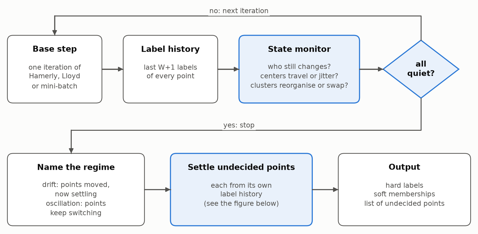
The base algorithm runs as usual while the recent labels of every point are kept. After each iteration a monitor asks three questions about the whole run, cheapest first. Once all three answers are quiet, the run stops.
| check | question | quiet when |
|---|---|---|
| Movement | Who still changes cluster? | almost no point changes, the changes are dying out, or the same points keep switching in steady numbers |
| Representatives | Are the centers travelling, or jittering in place? | the centers barely move, or only jitter around fixed positions |
| Partitions | Are the clusters reorganising, or only swapping members? | cluster sizes are steady, and few members move or they move both ways |
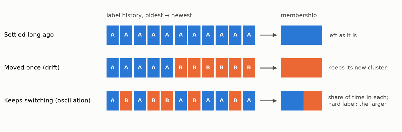
At the stop the monitor names the regime, and every undecided point is settled from its own label history:
| regime | what the undecided points do | how they are settled |
|---|---|---|
| drift | moved and are settling | a point that moved once keeps its new cluster; a point that went back and forth gets its share of time in each cluster |
| oscillation | keep switching forever | every point gets its share of time in each cluster; the larger share is its hard label |
Where the time of a run goes
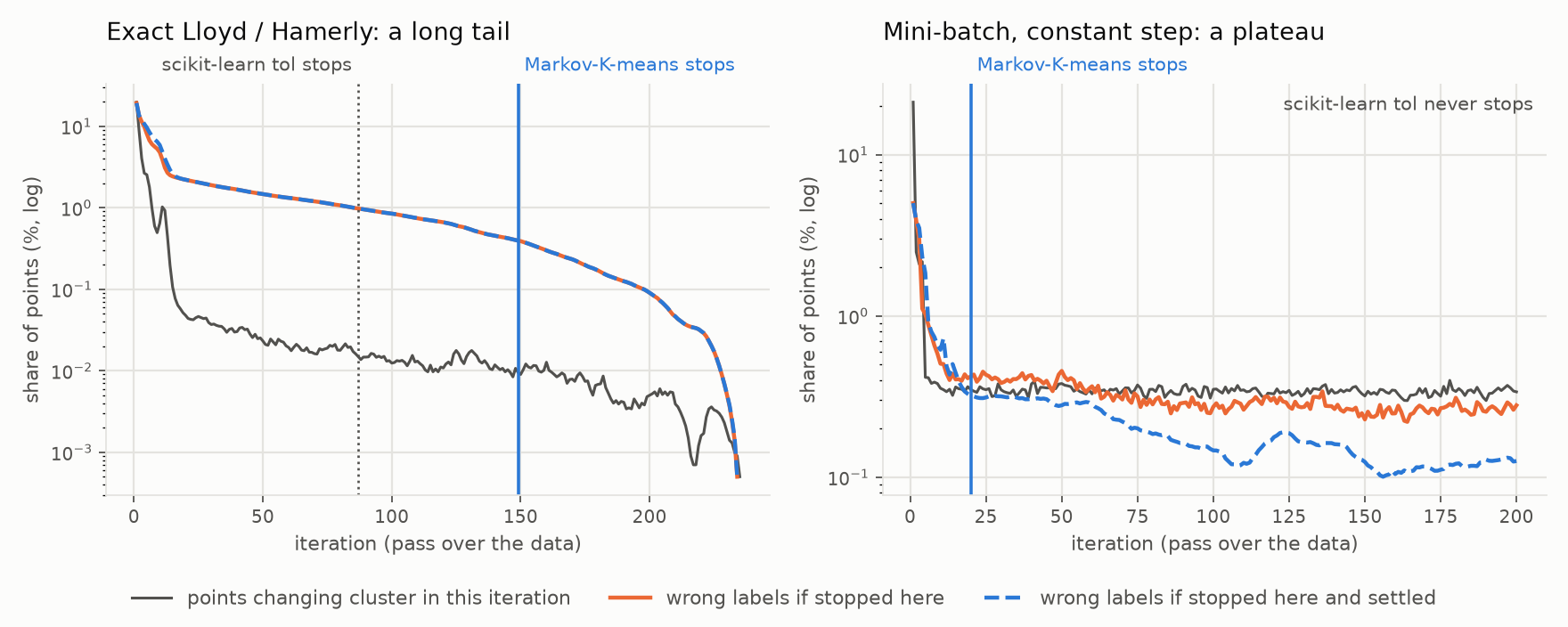
Exact Lloyd (left). After the early iterations only a tiny share of points still change cluster, yet the run goes on for many more passes over the data. That tail is what Markov-K-means cuts. Under drift, settling gives the same labels as stopping and keeping them (the two lines overlap), so the whole gain is the time saved.
Constant step (right). After a quick drop, the number of changing points stops falling. The run sits on a plateau, and the share of wrong labels barely moves however long it runs. Once on the plateau, settling the switching points from their history (dashed) leaves fewer wrong labels than keeping the current ones, and the gap widens as the run goes on. The automatic rule stops as soon as the plateau is reached. A later fixed stop (t0) with settlement buys a lower error for more time.
Time versus error, compared with other stopping rules
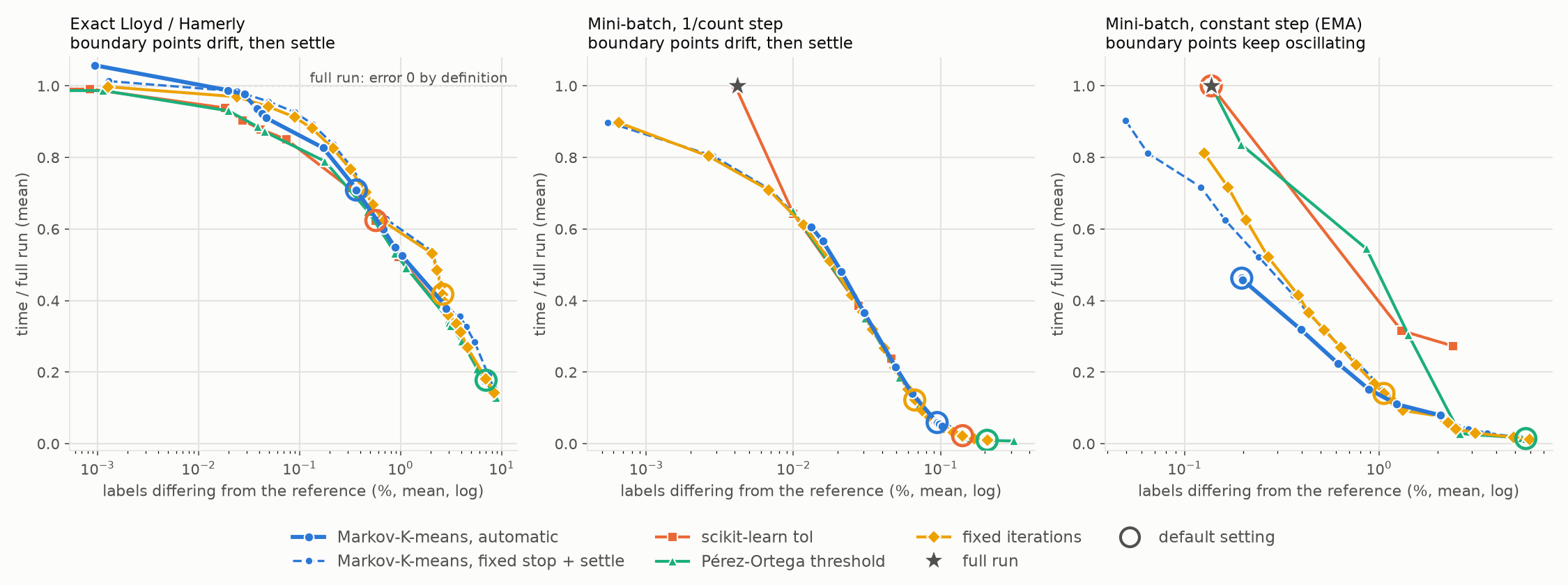
Each line is one stopping rule with its own setting swept. Every setting is applied unchanged to all datasets of a panel, as a user would choose it without knowing the outcome. A point gives the average error (labels that differ from the reference partition) and the average time relative to running to the end. Lower and further left is better. Circles mark the default settings.
| constant step / EMA | 1/count mini-batch | exact Lloyd / Hamerly | |
|---|---|---|---|
| Markov-K-means, automatic | fastest at every error level it reaches | among the fastest for precise answers; slower for rough ones, because it first watches a full window | on the shared curve, slightly behind a tuned threshold |
| Markov-K-means, fixed stop + settle | the only rule that goes below the full run's error | on the shared curve | slightly above the shared curve |
scikit-learn tol |
never stops at its default | on the shared curve | on the shared curve; slightly ahead when tuned |
| Pérez-Ortega threshold | stops too early or too late | on the shared curve | on the shared curve; slightly ahead when tuned |
| fixed iterations | stops at an arbitrary moment of the oscillation | on the shared curve | on the shared curve |
| where the defaults land | Markov-K-means: low error; scikit-learn: runs to the end; Pérez-Ortega: fast but rough | all at low error and little time | Markov-K-means and scikit-learn: low error; Pérez-Ortega and fixed iterations: fast but rough |
In short, each unit of error costs Markov-K-means the least time when training oscillates. With 1/count mini-batch it costs about the same as the other rules, and on exact Lloyd slightly more than a threshold tuned for the data.
Where it applies
| base algorithm | boundary points | what Markov-K-means adds |
|---|---|---|
exact Lloyd: "hamerly" (default), "lloyd" |
drift, then settle | cuts the tail without a tuned threshold; lists the undecided points |
1/count mini-batch, as in scikit-learn's MiniBatchKMeans: "minibatch" |
drift, then settle | the same |
constant-step mini-batch, the same update as an EMA codebook: "minibatch" with learning_rate="constant" |
keep oscillating | knows when to stop; labels better than the run's last state; memberships that mean share of time |
any other iterative hard assignment: assign_from_history |
either | settles each point from the recorded history |
Other iterative hard assignments include online or streaming k-means, VQ codebook training, and k-medoids or k-modes style reassignment. Record the labels at each step and pass them in:
from markov_kmeans import assign_from_history

r = assign_from_history(history)        # history: (n_steps, n_points), oldest first
r.labels, r.dense(n_clusters), r.uncertainty
When to use it
| situation | what you get |
|---|---|
| Large data with a long convergence tail | The tail is cut without tuning. The result differs from the converged one only on a few boundary points. |
| Constant-step, EMA or online training | A stopping point that no other rule finds. Labels better than the run's last state, and memberships that reflect time spent in each cluster. |
| You need to know which points are uncertain | A list of undecided points with soft memberships, ready for review, a more expensive model, or a downstream step that accepts soft assignments. |
| One setting must serve many datasets | Defaults that stay near the best trade-off whether the run drifts or oscillates. |
When not to use it
| situation | what goes wrong | use instead |
|---|---|---|
| Small or easy data | Monitoring and the observation window are pure overhead; the run is slightly slower than plain K-means. | plain K-means |
| Exact Lloyd with a threshold already tuned for this kind of data | The tuned threshold is slightly cheaper for the same error. | the tuned threshold |
| Only aggregate quality matters: colour palettes, inertia, compression quality | The aggregate settles long before individual points do, but the rule waits for the points. | fit on a sample, or a short fixed run |
| Codebooks that jitter strongly, such as EMA VQ codebooks in image tokenizers | The rule rightly never intervenes, so monitoring costs time and saves nothing. | plain training; distance-based soft tokens |
| You need the exact converged partition | It stops early by design. | run to convergence |
| A rough answer from 1/count mini-batch | Waiting for the observation window costs more than it saves. | a short fixed number of epochs |
Reading the soft membership
regime_ |
a fractional membership means | use it as |
|---|---|---|
"drift" |
the point is still undecided and will end in one cluster | a flag for points likely to be wrong |
"oscillation" |
the point really alternates, and the fractions match its long-run share of time | a soft assignment |
Limits
- The rule only sees what has happened so far. A point that looks settled at the stop but would move later is not caught, and most of the error left after a drift comes from such points. In the left panel above, wrong labels far outnumber changing points. A smaller
unstable_tolstops later and leaves fewer of them. - New points get the nearest center from
predict, since they have no history.
Main parameters
| parameter | default | meaning |
|---|---|---|
n_clusters |
8 | number of clusters |
algorithm |
"hamerly" |
"hamerly", "lloyd", "minibatch" |
learning_rate, eta, batch_size |
"count", 2e-4, 4096 |
mini-batch step: "count" (1/count) or "constant" (fixed eta) |
stop_rule |
"auto" |
"auto" judges the state; "unstable" looks only at the share of changing points |
assign_rule |
"auto" |
"auto" (by regime), "markov", "frequency", "keep" |
t0 |
None |
stop at this iteration instead, then settle |
unstable_tol |
1e-3 | lower stops later and leaves fewer undecided points |
window |
10 | iterations of label history kept per point |
min_iter, max_iter |
10, 300 | iteration bounds |
center_update |
"auto" |
final centers: "hard", "soft" (membership-weighted), "none" |
The monitor's other thresholds are documented in the docstring; the evaluation used their defaults. assign_rule="markov" settles every undecided point by the long-run law of its label Markov chain. Diagnostics include n_iter_, stop_reason_, regime_, decision_trace_, unstable_fraction_, n_dist_, fit_seconds_ and labels_at_stop_. MarkovKMeans is a scikit-learn estimator: it passes scikit-learn's check_estimator and works with clone, Pipeline, GridSearchCV and set_output.
Further reading
- Evaluation report: methods, every number behind the figures, colour quantization and VQ codebook studies
- Prior work
- Quick start
- Citing: CITATION.cff, or "Cite this repository" on the GitHub page
한국어
작동 방식
기반 알고리즘은 평소처럼 돌고, 모든 점의 최근 라벨이 기록된다. 매 반복 뒤 감시기가 실행 전체에 대해 세 가지를 묻는다. 싼 질문부터 묻고, 셋 다 잠잠해지면 멈춘다.
| 검사 | 질문 | 잠잠하다고 보는 때 |
|---|---|---|
| 움직임 | 아직 군집을 바꾸는 점은? | 바뀌는 점이 거의 없거나, 변화가 잦아들고 있거나, 같은 점들이 일정한 수로 계속 오갈 때 |
| 대표점 | 대표점이 이동 중인가, 제자리에서 흔들리기만 하는가? | 대표점이 거의 움직이지 않거나, 고정된 위치 주변에서 흔들리기만 할 때 |
| 분할 | 군집이 재편되는 중인가, 구성원을 주고받기만 하는가? | 군집 크기가 일정하고, 움직이는 구성원이 적거나 양방향으로 오갈 때 |
멈추면 감시기가 체제를 판정하고, 미결정 점은 각자의 라벨 이력으로 정리한다.
| 체제 | 미결정 점의 거동 | 정리 방식 |
|---|---|---|
| 표류 (drift) | 옮겨 가서 자리 잡는 중 | 한 번 옮긴 점은 새 군집에 두고, 왔다 갔다 한 점은 군집별로 머문 시간의 비율을 준다 |
| 진동 (oscillation) | 영원히 오감 | 모든 점에 군집별로 머문 시간의 비율을 주고, 더 큰 쪽을 hard 라벨로 삼는다 |
실행 시간은 어디에 쓰이는가
exact Lloyd (왼쪽). 초반 반복이 지나면 군집을 바꾸는 점은 아주 적은데, 실행은 그 뒤로도 데이터를 여러 번 더 훑는다. Markov-K-means가 끊는 것이 이 꼬리다. 표류 체제에서는 정리 결과가 멈춘 시점의 라벨을 그대로 두는 것과 같다(두 선이 겹친다). 이득은 전부 줄어든 시간에서 나온다.
고정 학습률 (오른쪽). 초반에 빠르게 줄어든 뒤로는 바뀌는 점의 수가 더 줄지 않는다. 실행은 평탄 구간에 머물고, 틀린 라벨의 비율은 아무리 오래 돌려도 거의 그대로다. 평탄 구간에서는 오가는 점을 이력으로 정리하면(점선) 현재 라벨을 그대로 둘 때보다 틀린 라벨이 적고, 그 차이는 실행이 길어질수록 벌어진다. 자동 규칙은 평탄 구간에 들어서자마자 멈춘다. 더 늦은 고정 시점(t0)에서 멈추고 정리하면 시간을 더 쓰는 대신 오차가 더 낮아진다.
다른 정지 규칙과 비교한 시간–오차 교환
선 하나는 정지 규칙 하나다. 각 규칙의 설정값을 바꿔 가며 돌렸고, 설정 하나는 한 패널의 모든 데이터에 그대로 적용했다. 결과를 모르는 사용자가 설정을 고르는 상황을 그대로 재현한 것이다. 점의 위치는 평균 오차(기준 분할과 라벨이 다른 점의 비율)와 평균 시간(끝까지 돌린 시간 대비)이다. 아래·왼쪽일수록 좋다. 동그라미는 각 규칙의 기본 설정이다.
| 고정 학습률 / EMA | 1/count mini-batch | exact Lloyd / Hamerly | |
|---|---|---|---|
| Markov-K-means 자동 규칙 | 닿는 모든 오차 수준에서 가장 빠름 | 정밀한 답에서 가장 빠른 축. 먼저 관찰 창 동안 지켜봐야 해서 대략적인 답에서는 느림 | 공통 곡선 위, 조정된 임계값보다 조금 뒤 |
| Markov-K-means 고정 정지 + 정리 | 끝까지 돌린 결과보다 낮은 오차에 닿는 유일한 규칙 | 공통 곡선 위 | 공통 곡선보다 조금 위 |
scikit-learn tol |
기본값에서 끝내 멈추지 못함 | 공통 곡선 위 | 공통 곡선 위, 조정하면 조금 앞섬 |
| Pérez-Ortega 임계값 | 너무 이르거나 너무 늦게 멈춤 | 공통 곡선 위 | 공통 곡선 위, 조정하면 조금 앞섬 |
| 고정 반복 수 | 진동 중 아무 순간에나 멈춤 | 공통 곡선 위 | 공통 곡선 위 |
| 기본값의 위치 | Markov-K-means: 낮은 오차. scikit-learn: 끝까지 돎. Pérez-Ortega: 빠르지만 거침 | 모두 낮은 오차, 적은 시간 | Markov-K-means와 scikit-learn: 낮은 오차. Pérez-Ortega와 고정 반복: 빠르지만 거침 |
정리하면, 오차 한 단위를 줄이는 데 드는 시간은 진동하는 학습에서 Markov-K-means가 가장 적다. 1/count mini-batch에서는 다른 규칙과 비슷하고, exact Lloyd에서 데이터에 맞춰 조정한 임계값과 비교하면 조금 더 든다.
적용 가능한 알고리즘
| 기반 알고리즘 | 경계 점의 거동 | Markov-K-means가 더하는 것 |
|---|---|---|
exact Lloyd: "hamerly"(기본), "lloyd" |
표류 후 정착 | 임계값 조정 없이 꼬리를 끊고, 미결정 점 목록을 준다 |
scikit-learn MiniBatchKMeans와 같은 1/count mini-batch: "minibatch" |
표류 후 정착 | 위와 같다 |
EMA 코드북과 같은 고정 보폭 mini-batch: "minibatch", learning_rate="constant" |
계속 진동 | 언제 멈출지 알고, 마지막 상태보다 나은 라벨과 머문 시간 비율로서의 소속도를 준다 |
그 밖의 반복형 hard 배정: assign_from_history |
둘 다 | 기록된 이력으로 각 점을 정리한다 |
그 밖의 반복형 hard 배정에는 온라인·스트리밍 k-means, VQ 코드북 학습, k-medoids·k-modes식 재배정이 있다. 매 단계의 라벨을 기록해 넘기면 된다.
from markov_kmeans import assign_from_history

r = assign_from_history(history)        # history: (단계 수, 점 수), 오래된 단계부터
r.labels, r.dense(n_clusters), r.uncertainty
이럴 때 쓰면 좋다
| 상황 | 얻는 것 |
|---|---|
| 수렴 꼬리가 긴 대용량 데이터 | 조정 없이 꼬리가 끊긴다. 결과는 수렴한 결과와 경계의 소수 점에서만 다르다. |
| 고정 학습률, EMA, 온라인 학습 | 다른 규칙이 찾지 못하는 정지 시점을 얻는다. 라벨은 마지막 상태보다 정확하고, 소속도는 군집별로 머문 시간을 나타낸다. |
| 어떤 점이 불확실한지 알아야 할 때 | soft 소속도가 붙은 미결정 점 목록을 얻는다. 사람 검토, 더 비싼 모델, soft 배정을 받는 후속 단계로 바로 넘길 수 있다. |
| 설정 하나로 여러 데이터를 처리해야 할 때 | 표류든 진동이든 최적 교환선 가까이에 놓이는 기본값을 쓸 수 있다. |
이럴 때는 오히려 독이 된다
| 상황 | 무엇이 문제인가 | 대신 쓸 것 |
|---|---|---|
| 작거나 쉬운 데이터 | 감시와 관찰 창이 순수한 추가 비용이 되어, 그냥 K-means보다 약간 느리다. | 그냥 K-means |
| 같은 종류의 데이터에 맞춰 임계값을 이미 조정해 둔 exact Lloyd | 같은 오차를 조정된 임계값이 조금 더 싸게 얻는다. | 조정된 임계값 |
| 색 팔레트, inertia, 압축 화질처럼 전체 품질만 중요할 때 | 집계 지표는 점들보다 훨씬 먼저 안정되는데, 규칙은 점 하나하나를 기다린다. | 표본 학습, 짧은 고정 반복 |
| 이미지 토크나이저의 EMA VQ 코드북처럼 크게 흔들리는 코드북 | 규칙이 개입하지 않는 것이 옳으므로, 감시 비용만 들고 절감은 없다. | 일반 학습, 거리 기반 soft 토큰 |
| 정확히 수렴한 분할이 필요할 때 | 설계상 일찍 멈춘다. | 끝까지 수렴 |
| 1/count mini-batch로 대략적인 답만 필요할 때 | 관찰 창을 기다리는 비용이 아끼는 시간보다 크다. | 짧은 고정 epoch |
soft 소속도 읽는 법
regime_ |
분수형 소속도의 뜻 | 쓰는 법 |
|---|---|---|
"drift" |
아직 미결정이고, 결국 한 군집에 정착한다 | 틀릴 가능성이 큰 점의 표시 |
"oscillation" |
실제로 오가며, 비율이 장기적으로 머무는 시간과 맞는다 | soft 배정 |
한계
- 판단은 지금까지 관찰한 것만으로 내린다. 멈출 때 자리 잡은 듯 보였다가 나중에 옮겨 갈 점은 잡지 못하고, 표류 뒤 남는 오차는 대부분 이런 점에서 나온다. 위 왼쪽 그림에서 틀린 라벨이 바뀌는 점보다 훨씬 많은 이유다.
unstable_tol을 낮추면 더 늦게 멈추는 대신 이런 점이 줄어든다. - 새 점은 이력이 없으므로
predict가 가장 가까운 대표점을 준다.
주요 매개변수
| 매개변수 | 기본값 | 의미 |
|---|---|---|
n_clusters |
8 | 군집 수 |
algorithm |
"hamerly" |
"hamerly", "lloyd", "minibatch" |
learning_rate, eta, batch_size |
"count", 2e-4, 4096 |
mini-batch 보폭: "count"(1/count) 또는 "constant"(고정 eta) |
stop_rule |
"auto" |
"auto"는 상태를 판정하고, "unstable"은 바뀌는 점의 비율만 본다 |
assign_rule |
"auto" |
"auto"(체제별), "markov", "frequency", "keep" |
t0 |
None |
이 반복에서 멈춘 뒤 정리한다 |
unstable_tol |
1e-3 | 낮출수록 늦게 멈추고 미결정 점이 줄어든다 |
window |
10 | 점마다 보관하는 라벨 이력의 반복 수 |
min_iter, max_iter |
10, 300 | 반복 수 범위 |
center_update |
"auto" |
최종 대표점: "hard", "soft"(소속도 가중), "none" |
감시기의 나머지 임계값은 docstring에 정리되어 있고, 평가는 모두 기본값으로 했다. assign_rule="markov"는 모든 미결정 점을 라벨 Markov 연쇄의 장기 분포로 정리한다. 진단 속성으로 n_iter_, stop_reason_, regime_, decision_trace_, unstable_fraction_, n_dist_, fit_seconds_, labels_at_stop_이 있다. MarkovKMeans는 scikit-learn 추정기다. scikit-learn의 check_estimator를 통과하고 clone, Pipeline, GridSearchCV, set_output과 함께 쓸 수 있다.
더 보기
- 평가 보고서: 방법, 그림 뒤의 모든 수치, 색 양자화·VQ 코드북 실험
- 선행연구
- 빠른 시작 예제
- 인용: CITATION.cff 또는 GitHub 페이지의 "Cite this repository"
Apache-2.0
1 maintainer

Metadata
1 maintainer
Release files for markov-kmeans 0.3.0
For a detailed explanation of source distributions (sdists) and built distributions (wheels), please see the package formats documentation.
Source distribution (sdist)
| File | Size | Uploaded | |
|---|---|---|---|
| markov_kmeans-0.3.0.tar.gz | 37.3 kB | Details |
Built distribution (wheel)
| File | Interpreter | ABI | Platform | Reset |
|---|---|---|---|---|
| markov_kmeans-0.3.0-py3-none-any.whl | Python 3 | none | any | Details |
Total release size: 69.0 kB
Release files / markov_kmeans-0.3.0.tar.gz
| Download URL | markov_kmeans-0.3.0.tar.gz |
|---|---|
| Size | 37.3 kB |
| Tags | Source |
|
SHA-256 checksum How to use checksums |
3c303cc076aa1e18c2d77bc76b452461c25b4ecfb682940ddc998d02a3dd431e
|
|
BLAKE2b-256 checksum How to use checksums |
c9e4a3d21d3fa24198fbc0df17441801684ff4420e94562264bd74cb4473b351
|
| Upload date | |
|
Uploaded using Trusted Publishing? What is trusted publishing? |
Yes |
| Uploaded via |
twine/7.0.0 CPython/3.13.14
|
Provenance
Provenance describes where a file came from. On PyPI, provenance is shared via attestations, which provide a verifiable record of the build or publishing details. View details, limitations and caveats.


PyPI Publish Attestation
PyPI verified that this artifact, at this checksum, originated from the publisher listed below.
Signed by GitHub Actions, verified by PyPI on Oct 3, 2026.
Transparency logRelease files / markov_kmeans-0.3.0-py3-none-any.whl
| Download URL | markov_kmeans-0.3.0-py3-none-any.whl |
|---|---|
| Size | 31.7 kB |
| Tags | Python 3 |
|
SHA-256 checksum How to use checksums |
ffe1f5f7f14ee23e2884c28baff69a6de466efea8abd62a7aebae8595c6f4037
|
|
BLAKE2b-256 checksum How to use checksums |
7fd8d928af5210b2d5bbace6b08e3bc3230745895ad35dbe9dbc070d5f491dd2
|
| Upload date | |
|
Uploaded using Trusted Publishing? What is trusted publishing? |
Yes |
| Uploaded via |
twine/7.0.0 CPython/3.13.14
|
Provenance
Provenance describes where a file came from. On PyPI, provenance is shared via attestations, which provide a verifiable record of the build or publishing details. View details, limitations and caveats.
PyPI Publish Attestation
PyPI verified that this artifact, at this checksum, originated from the publisher listed below.
Signed by GitHub Actions, verified by PyPI on Oct 3, 2026.
Transparency log













