
Bühlmann-Splinter Decompression Algorithm
The Bühlmann decompression algorithm is a widely used model in scuba diving to calculate safe ascent profiles, based on inert gas (mainly nitrogen or helium) uptake and elimination in human tissues.
The algorithm was developed by Dr. Albert A. Bühlmann, a Swiss physician and researcher at the University of Zürich. His work led to a series of decompression models, culminating in the ZHL-16 model, which uses 16 parallel tissue compartments with different half-times. These models form the basis of many modern dive computers and decompression tables used by recreational and technical divers.
The foundational research is described on:
Bühlmann, A. A.(1983). Decompression–Decompression Sickness. Springer-Verlag,ISBN: 978-3540127576
"Dekompression – Dekompressionskrankheit"
Contents
- Installation — what to install, and what you get
- Quick look — the smallest thing that does something
- Methodology — the model, its equations, its sea level reference, and a worked dive
- Using the Model Directly — the library's public surface
- Module A — Dive Profile Analyser — run a planned dive against the model
- Module B — Altitude Analyser — flying or driving to altitude afterwards
- Project layout — how the four layers sit
- Regenerating the Report Graphs — reproducing everything in
reports/
Installation
Python 3.11 or newer, and no runtime dependencies — the library imports nothing outside the standard library.
pip install master-splinter
That gives you the model and nothing else: no commands, no file formats of its own, and no opinion about where your data lives. A front end supplies those, and Using the Model Directly is the whole surface it drives.
To work on the project, from a checkout:
pip install -e '.[dev,test]'
The dev extra adds matplotlib, which nothing in the library needs — only tools/methodology_figures.py and the two commands in cli/ draw anything.
Quick look
Plan a dive, execute it against the model, and see what it costs you:
from master_splinter.model.dive_state import DiveState
from master_splinter.processors.dive_analysis import analyse_profile
from master_splinter.processors.dive_simulation import generate_dive_profile

profile = generate_dive_profile([
    (30, 2, (0, 0), "descend"),    # 30 m over 2 min
    (30, 25, (0, 0), "constant"),  # 25 min on the bottom
    (0, 3, (0, 0), "ascend"),      # up in 3 min
])
report = analyse_profile(profile, DiveState.at_surface())

for stop in report.stops:
    print(f"{stop.depth:.0f} m for {stop.duration:.1f} min")
print(f"{report.total_deco_time:.1f} min of decompression")
6 m for 3.2 min
3 m for 6.5 min
9.7 min of decompression
That three-minute ascent was never going to happen: analyse_profile clamps to
the decompression ceiling and reports the stops the clamping forced. The rest
of that surface is in Using the Model Directly;
why those are the stops is Methodology.
Methodology
Why the numbers above are the numbers they are. The four sections below are the tissue table, the equations that drive it, the sea level reference they are all measured against, and a worked example small enough to follow by hand.
ZHL-16 Tissue Compartment Table with Tissue Types
The ZHL-16 tissue table lists 16 mathematical compartments that represent different types of body tissues — each with its own half-time, and parameters A and B that determine its decompression limits.
Variant: this implementation uses the
ZHL-16Ccoefficients, the set most dive computers ship.
Bühlmannpublished three.ZHL-16Ais the original theoretical set, in which both coefficients fall straight out of the half-time —a = 2 / ∛Tandb = 1.005 − 1/√T. It proved too permissive against real data, so he revised the mid and slowAvalues by hand, givingZHL-16Bfor printed tables andZHL-16Cfor dive computers. TheBvalues were never revised and are identical in all three sets, which is the quickest way to spot a corrupted table.Both sets live in
src/master_splinter/configs/zhl16.py, so changing variant really is the single edit that file claims.16Ais materially more permissive — on a30 m / 60 mindive it asks for about a fifth less decompression.
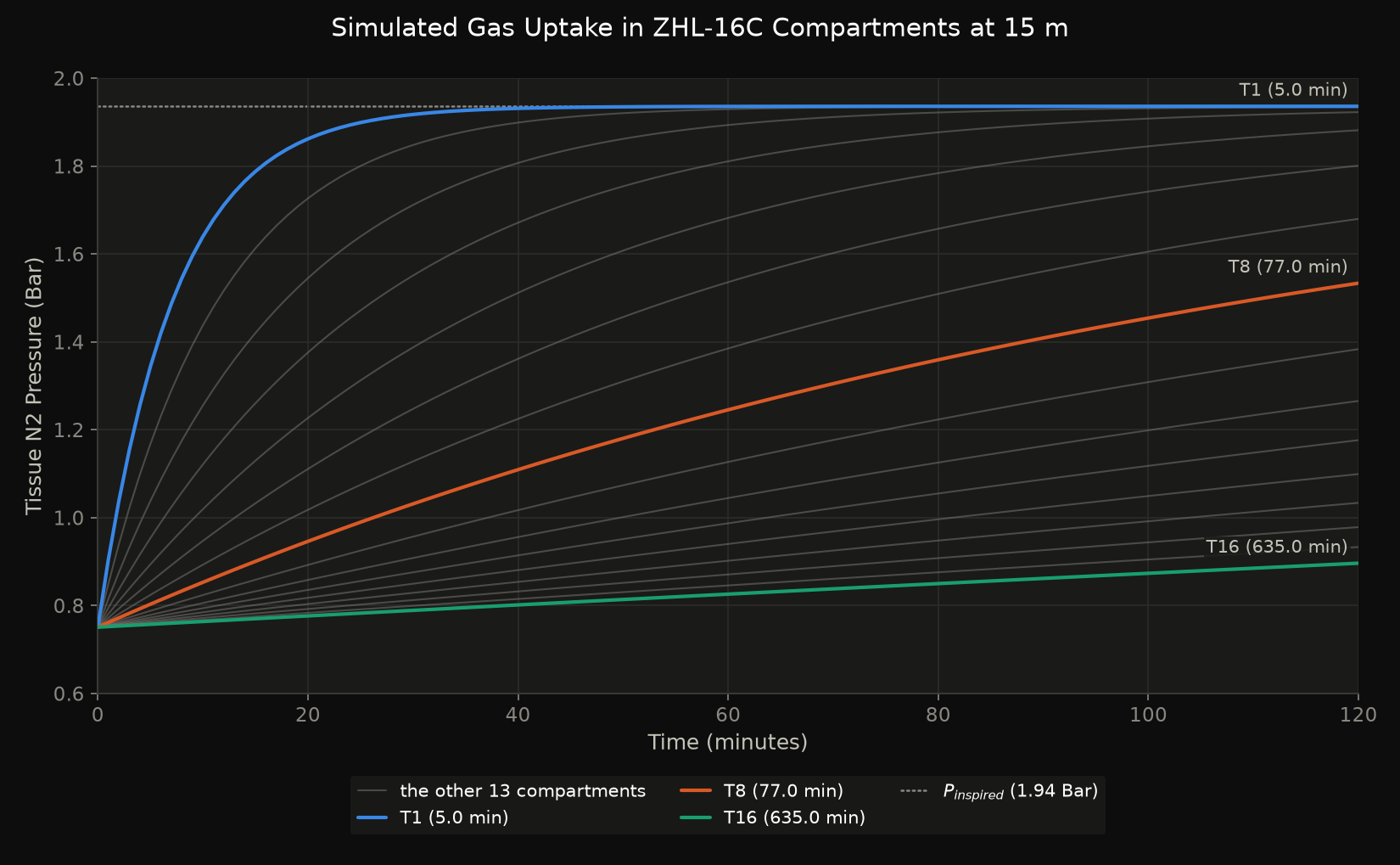
These compartments are not actual organs, but conceptual models that simulate how inert gases (e.g. nitrogen or helium) are absorbed and released in different parts of the body at different rates.
| # | Half-Time (in minutes) | A-Value | B-Value | Tissue Type | Notes |
|---|---|---|---|---|---|
| 1 | 5.0 |
1.1696 |
0.5578 |
Blood/Plasma |
Very fast |
| 2 | 8.0 |
1.0000 |
0.6514 |
Lungs |
Fast |
| 3 | 12.5 |
0.8618 |
0.7222 |
Skin |
|
| 4 | 18.5 |
0.7562 |
0.7825 |
Brain |
|
| 5 | 27.0 |
0.6200 |
0.8126 |
Muscle (active) |
|
| 6 | 38.3 |
0.5043 |
0.8434 |
Muscle (deep) |
|
| 7 | 54.3 |
0.4410 |
0.8693 |
Organs |
Medium |
| 8 | 77.0 |
0.4000 |
0.8910 |
Organs |
|
| 9 | 109.0 |
0.3750 |
0.9092 |
Fat (shallow) |
|
| 10 | 146.0 |
0.3500 |
0.9222 |
Fat (medium) |
|
| 11 | 187.0 |
0.3295 |
0.9319 |
Fat (deep) |
|
| 12 | 239.0 |
0.3065 |
0.9403 |
Bone (cancellous) |
|
| 13 | 305.0 |
0.2835 |
0.9477 |
Bone (dense) |
Slow |
| 14 | 390.0 |
0.2610 |
0.9544 |
Bone |
|
| 15 | 498.0 |
0.2480 |
0.9602 |
Fat/Bone |
|
| 16 | 635.0 |
0.2327 |
0.9653 |
Fat/Bone |
Very slow |
Half-Time: Time (in minutes) it takes the tissue to absorb or release 50% of the inert gas differenceA-Value: Intercept in theM-valueequation — tolerance for supersaturation at surface pressureB-Value: Reciprocal of the slope in theM-valueequation —P_ambientis divided by it, so a lowerBmeans tolerance rises faster with depthTissue Type: Conceptual mapping to a body tissue (e.g. blood, muscle, fat, bone)Notes: Fast/slow behavior in decompression
A and B Values
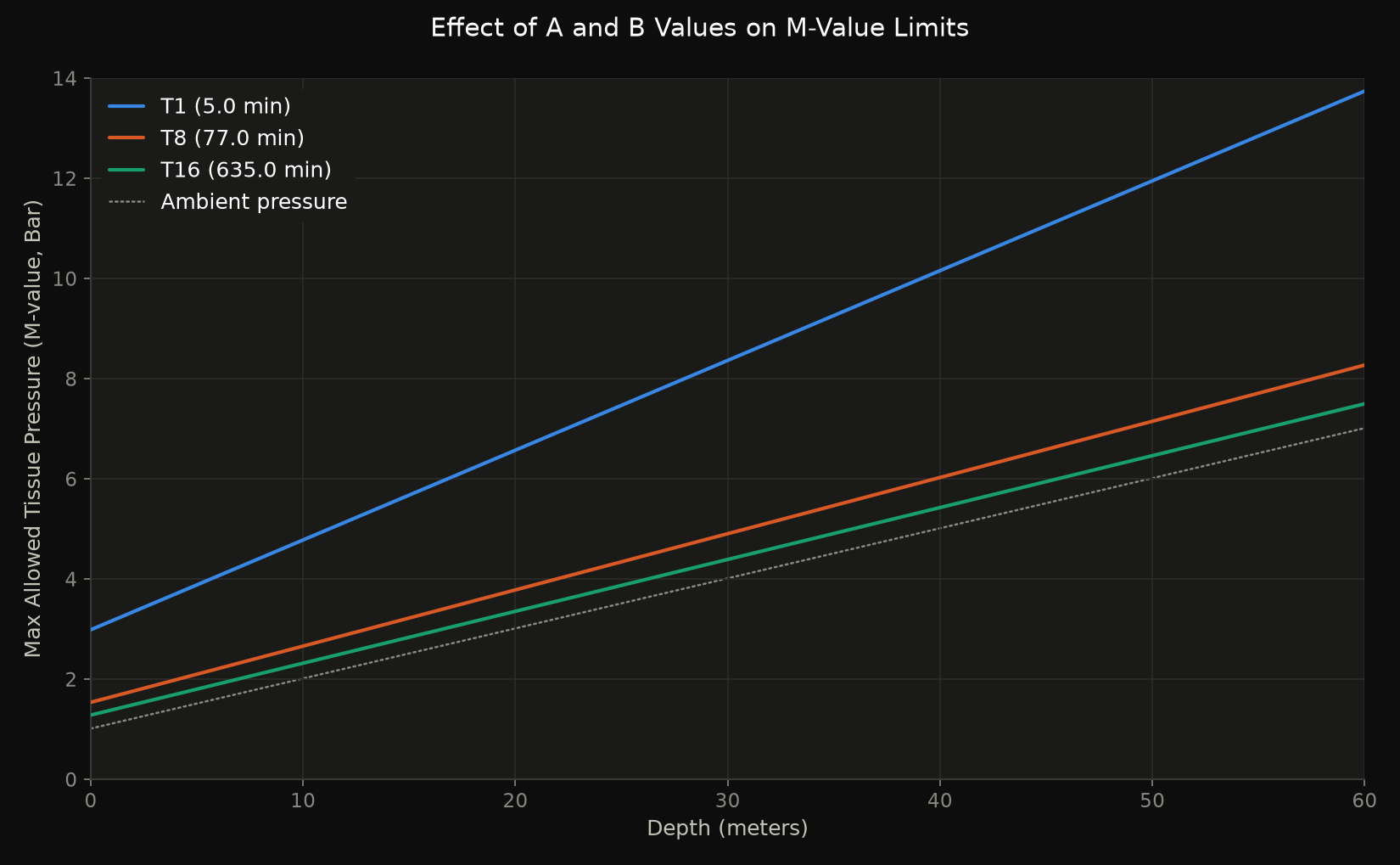
They are used to calculate the M-value, the maximum safe inert gas pressure in a tissue:
- A (
intercept): A constant that sets the baselinesupersaturationlimit for a tissue compartment at surface pressure - B (
reciprocal slope):P_ambientis divided byB, so a lowerBmakes theM-valueclimb more steeply with depth
Together, they define the ceiling for each tissue — i.e., how shallow the diver can go before needing a decompression stop.
| Tissue Type | Half-Time | A Value | B Value | Surfacing M-value |
Behavior at Depth |
|---|---|---|---|---|---|
| Fast | Low | High | Low | High (2.99 bar) |
Loads and clears quickly; tolerates the most supersaturation |
| Slow | High | Low | High | Low (1.28 bar) |
Loads slowly; tolerates the least supersaturation |
fast tissues (e.g., half-time 5–18 minutes)
Fast Tissues present lower B values (e.g., 0.5578 to 0.78). Because P_ambient is divided by B, their M-value climbs faster with depth, and compartment 1 tolerates 2.99 bar at the surface — the highest of the 16. They dominate the early part of an ascent because their short half-time loads them quickly, not because their limit is low.
slow tissues (e.g., 200–600+ minutes)
Slow Tissues present higher B values (e.g., 0.94 to 0.97). Their M-value climbs more slowly with depth and sits lowest at the surface (1.28 bar for compartment 16). They load slowly, but on long dives they become the limiting compartments and are what drive the long shallow stops.
Mathematical Foundations
This section summarizes the core equations behind the Bühlmann ZHL-16 decompression model, which simulates how inert gases (e.g., nitrogen or helium) are absorbed and eliminated from body tissues during a dive.
1. Tissue Gas Uptake and Elimination
Each tissue compartment follows a first‑order exponential model for gas loading and off‑gassing:
$$ \Large P_{\text{tissue}}(t) = P_{\text{tissue}}(0) + \left( P_{\text{inspired}} - P_{\text{tissue}}(0) \right) \left( 1 - e^{-kt} \right) $$
symbol definitions
Where:
P_tissue(t): inert gas pressure in the tissue after timetP_tissue(0): initial tissue gas pressureP_inspired: inspired inert gas pressure at a given depthk:ln(2) / half_time- it defines how fast a tissue absorbs or releases inert gashalf_time: tissue half‑time (in minutes)t: time at depth (in minutes)
This same equation is used for both:
- On‑gassing (when
P_inspired > P_tissue) - Off‑gassing (when
P_inspired < P_tissue)
2. Inspired Inert Gas Pressure
The inspired inert gas pressure is calculated from ambient pressure and gas fraction:
$$ \Large P_{\text{inspired}} = f_{\text{gas}} \cdot \left( P_{\text{ambient}} - P_{H_2O} \right) $$
symbol definitions
Where:
gas_fraction: fraction of inert gas (e.g.0.79for nitrogen in air)P_ambient: ambient pressure in bar (1.01325 + depth / 10)P_H2O: water vapor pressure in the lungs (0.0627 bar)
3. M‑Value (Maximum Safe Tissue Pressure)
Bühlmann defined a maximum allowable inert gas pressure (M‑value) for each tissue compartment:
$$ \Large M = \frac{P_{\text{ambient}}}{B} + A $$
symbol definitions
Where:
A: tissue‑specific intercept (ZHL16_Avalue)B: tissue‑specific reciprocal slope (ZHL16_Bvalue) —P_ambientis divided by itP_ambient: ambient pressure in barM: maximum safe tissue pressure at that depth
If the tissue pressure exceeds
M, a decompression stop is required.
4. Ascent Ceiling (Minimum Ambient Pressure)
To calculate the shallowest depth a diver can safely ascend to, the M‑value equation is rearranged:
$$ \Large P_{\text{ambient}}^{\min} = \left( P_{\text{tissue}} - A \right) \cdot B $$
symbol definitions
Where:
P_tissue: current inert gas pressure in the tissueP_ambient_min: minimum safe ambient pressure
This value defines the decompression ceiling.
5. Gradient Factors
Gradient Factors add conservatism by scaling down the M‑value:
$$ \Large P_{\text{allowed}} = P_{\text{ambient}} + GF \cdot \left( M - P_{\text{ambient}} \right) $$
Since GF lies between 0 and 1, the allowed pressure always falls between ambient pressure and the raw M-value — a gradient factor can only ever scale the allowance down. Its value is interpolated across the ascent, from GF_low at the first stop to GF_high at the surface:
$$ \Large GF = GF_{\text{high}} - \left( GF_{\text{high}} - GF_{\text{low}} \right) \cdot \frac{P_{\text{ambient}} - P_{\text{surface}}}{P_{\text{first stop}} - P_{\text{surface}}} $$
symbol definitions and gradient factor pairs
GF_low and GF_high are two values that define how conservative a decompression algorithm should be when calculating ascent ceilings and required stops.
Where:
GF: gradient factor between 0 and 1GF_low: applied at the deepest decompression stop. Forces the diver to stop deeper and earlier; it helps control bubble formation when tissues are most saturatedGF_high: applied near the surface. Controls how close tissue pressure can get to theM-valueat surfacing
Example:
GF_low= 30 → only allows30%of the way to the fullBühlmannlimit at the first deco stop.
Example:GF_high= 85 → allows85%of the fullBühlmannM-valueas the final tissue ceiling at surfacing.
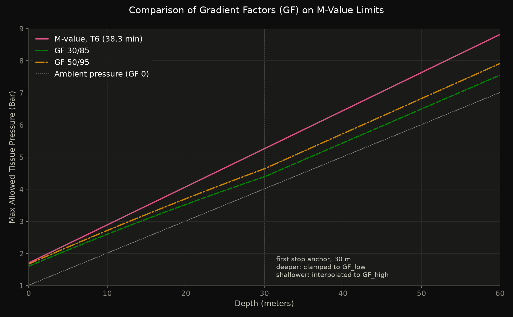
This graph compares conservative (GF
30/85) and less conservative (GF50/95) gradient factors, showing how each setting adjusts the safe tissue pressure ceiling below theBühlmannM-valueline across different depths. Both lines sit below theM-valueat every depth and above ambient pressure, which is theGF 0floor drawn dotted. The kink at30 mis the first stop anchor: deeper than it the factor is clamped toGF_low, shallower it interpolates towardsGF_high.
GF 100/100 allows surfacing as soon as no compartments exceed their raw M-value — it's efficient but higher risk if you're close to the limit.
GF_low |
GF_high |
Description |
|---|---|---|
30 |
85 |
Conservative default (common) |
50 |
95 |
Moderately aggressive |
100 |
100 |
Pure Bühlmann — no conservatism |
The effect of using gradient factors versus pure Bühlmann in a recreational dives up to 30 meters largely depends on how the dive is structured—particularly the bottom time and how the ascent is handled. For most no-decompression dives at this depth, the differences are usually minimal. If the diver ascends slowly and includes a standard safety stop, the added conservatism from gradient factors often doesn’t significantly alter the outcome. In these cases, tissue pressures typically remain well within safe limits, and both models would allow a clean ascent without requiring decompression stops.
The practical impact of GF only becomes noticeable in longer dives, more aggressive profiles, or when approaching decompression thresholds.
The Sea Level Reference
Every pressure above is absolute, in bar, and every one of them is measured against a sea level of 1.01325 bar — the published International Standard Atmosphere P0 (101325 Pa), set once as SURFACE_PRESSURE in src/master_splinter/configs/environment.py.
That is worth stating because most diving literature rounds it to 1 bar, and this project deliberately does not. The reason is the elevation conversion:
$$ \Large P(h) = P_0 \cdot \left( 1 - 2.25577 \times 10^{-5} \cdot h \right)^{5.25588} $$
Those two constants are calibrated as a set with P0 = 101325 Pa. Keeping them while rounding P0 to 1.0 gives a curve of the right shape through the wrong point — self-consistent, and wrong by about 110 m at every elevation:
| Elevation | Rounded P0 = 1.0 |
ISA P0 = 1.01325 |
|---|---|---|
0 m |
1.0000 bar |
1.0132 bar |
1,800 m |
0.8042 bar |
0.8149 bar |
2,400 m |
0.7464 bar |
0.7563 bar |
The middle column is a pressure that belongs to neither convention: it is 2,400 m on the diving scale and 2,505 m on the standard atmosphere. Since altitude analysis compares tissue pressures directly against these figures, the project uses the ISA value throughout so that a stated elevation means what it says.
The visible consequences are small and all of a piece — a sea level dive reports 1.0132 bar rather than 1.0000 bar, surface equilibrium is 0.7509 bar rather than the 0.7405 bar of the tables, and compartment 1's surfacing M-value is 2.99 bar rather than the tabulated 2.96 bar. Each is the same equation evaluated at a real sea level instead of a rounded one.
The published
ZHL-16CAandBcoefficients are unaffected. They are properties of the algorithm, not of the atmosphere, and are used exactly asBühlmannprinted them.
Simulating a Simple Dive
Here's how these formulas come together in a practical example of a typical dive simulation:
Dive Profile
- Descend to 15 meters (ambient pressure
≈ 2.513 bar) - Stay at 15 meters depth for 30 minutes
- Ascend to 5 meters and stay for 3 minutes
- Surface (ambient pressure
≈ 1.013 bar)
Step-by-Step Application
-
Calculate inspired nitrogen pressure at
15 meters:P_ambient= 1.01325 + (15 / 10) =2.513 barP_inspired= 0.79 × (2.513 − 0.0627)≈ 1.936 bar
-
Update each tissue using the gas loading formula for 30 minutes at 15m:
- For each of the
16 compartments:- Apply:
P_tissue(t) = P_tissue(0) + (P_inspired − P_tissue(0)) × (1 − e^(−k × t))
- Apply:
- For each of the
-
Ascend to
5 meters, recalculateP_inspired, and update tissue pressures again for3 minutes. -
Check each compartment before surfacing:
- Compute its
M-value:M = P_ambient / B + A - Compare to the current
P_tissue - If
P_tissue > M, decompression stop is required
- Compute its
-
(Optional) Apply Gradient Factors:
- Calculate a GF-adjusted limit:
P_allowed = P_ambient + GF × (M − P_ambient) - This helps determine whether it's safe to surface under conservative settings like GF
30/85
- Calculate a GF-adjusted limit:
Result
The dive simulation models a straightforward profile: a descent to 15 meters for 30 minutes, followed by a direct ascent to 5 meters with a 3-minute safety stop, and then surfacing. The fast compartment is the one that visibly does the work — it loads to 1.92 bar over the bottom phase and is already off-gassing by the safety stop, ending at 1.53 bar. The medium and slow compartments are still filling when the diver surfaces; on a dive this short they barely turn over at all, peaking at 1.04 and 0.79 bar respectively.
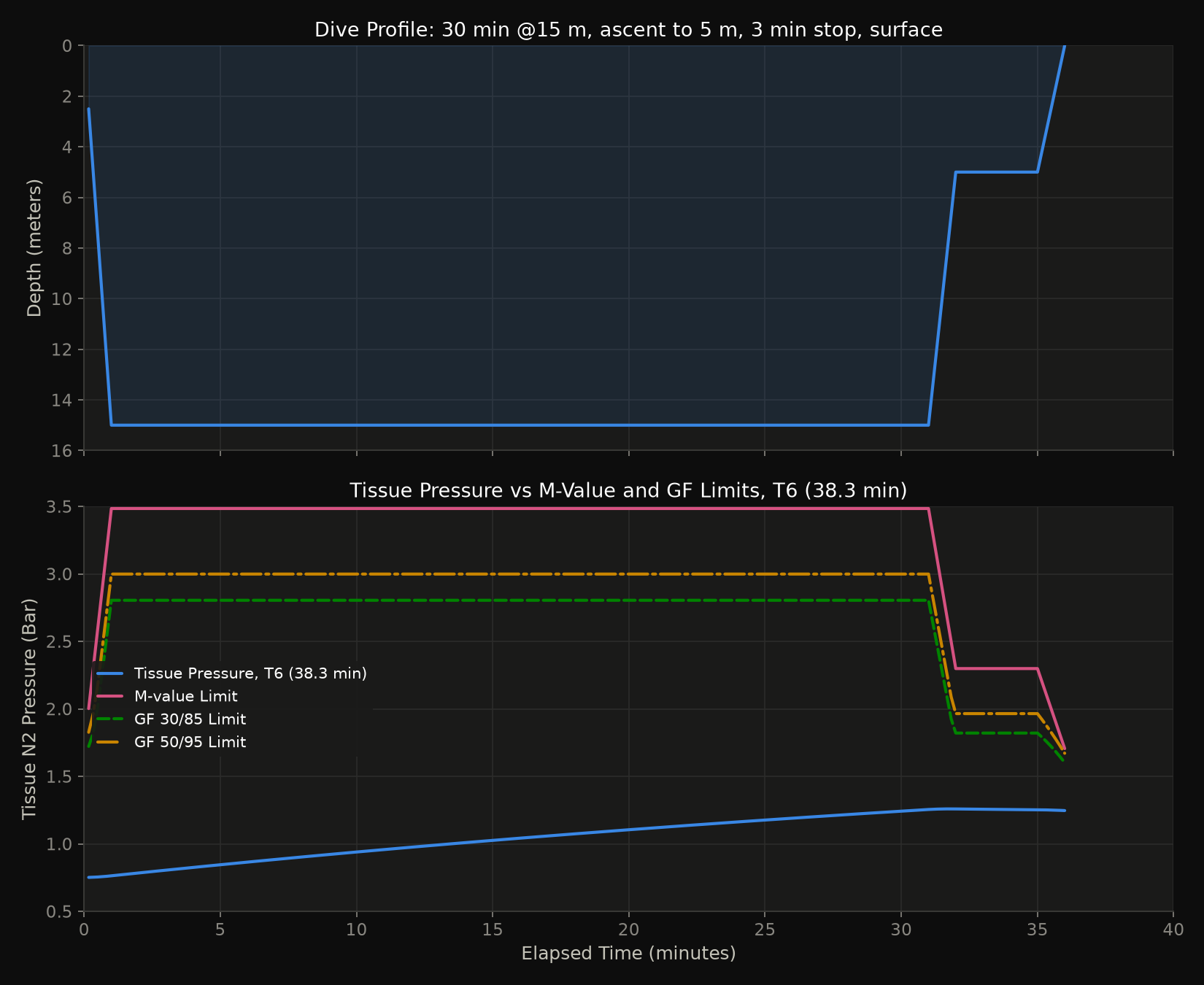
Using Bühlmann’s ZHL-16 algorithm, the tissue pressure remains safely below the calculated M-value limit. Two sets of gradient factors (GF 30/85 and GF 50/95) were applied to assess additional safety margins. The tissue pressure did not exceed either of these GF-adjusted ceilings at any point, indicating the diver stayed within conservative ascent limits.
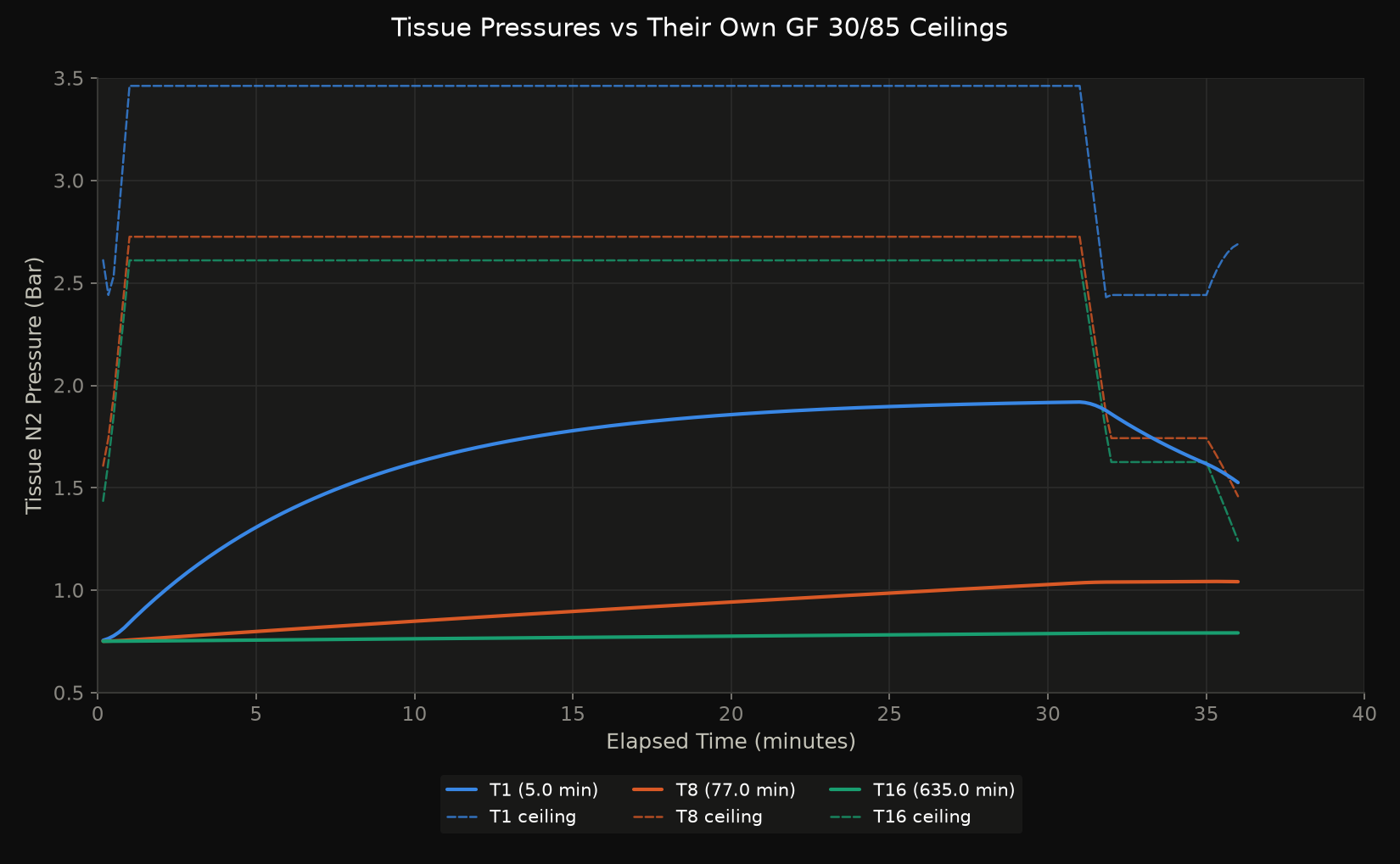
Each compartment is paired with its own
GF 30/85ceiling, in the same colour. Drawing one compartment's ceiling across all three would compare a pressure against a limit that was never its own.
The absence of any threshold crossings suggests that no decompression stop was required, and the 3-minute hold at 5 meters was sufficient to manage supersaturation before surfacing. Overall, this profile represents a clean, no-decompression dive that adheres well to both standard and conservative ascent protocols.
Using the Model Directly
DiveState carries the tissue loading and the gradient factor anchor, and is the object every entry point below drives.
Analysing a dive
The Quick look above, with what it left out. A profile is a list of (depth, duration, elapsed) tuples: generate_dive_profile builds one from phase boundaries, load_profile reads one from a dive computer log.
from master_splinter.model.dive_state import DiveState
from master_splinter.processors.dive_analysis import analyse_profile
from master_splinter.processors.dive_simulation import generate_dive_profile

profile = generate_dive_profile([
    (30, 2, (0, 0), "descend"),
    (30, 25, (0, 0), "constant"),
    (0, 3, (0, 0), "ascend"),
])

report = analyse_profile(profile, DiveState.at_surface(gas_fraction=0.79))
print(report.stops, report.total_deco_time, report.findings)
analyse_profile does not merely judge the plan — it executes it, clamping every ascent to the decompression ceiling. So report.samples is the dive that could actually be performed, not the one requested, and report.stops is what clamping forced. report.findings lists where the plan itself was unsafe, each tagged with a Violation:
from master_splinter.processors.dive_analysis import Violation

for finding in report.findings_of(Violation.ASCENT_RATE):
    print(finding)
The knobs are keyword-only: ascent_rate, deco_step, and ppo2_limit (bar, default 1.4, and never above PPO2_CONTINGENCY_LIMIT — see ppo2_limit below).
Going up afterwards
analyse_altitude_change answers the flying-after-diving question against the tissue state a dive ended on. The gain is measured relative to the dive site, which is why surface_pressure is a parameter rather than an assumption:
from master_splinter.processors.altitude_analysis import analyse_altitude_change

verdict = analyse_altitude_change(
    report.final_state.tissues,
    elevation_gain=2400,        # a pressurised cabin
    surface_interval=18 * 60,   # minutes since surfacing
    gf_high=0.85,
)
print(verdict.safe, verdict.gradient.wait_minutes, verdict.gradient.max_gain)
It reports two Verdicts side by side — raw for unmodified Bühlmann and gradient for the GF-limited answer — and report.safe is true only when both permit the change. When a verdict is unsafe, wait_minutes is the extra surface time needed, or None when no surface interval is ever enough.
This models tissue nitrogen only. It is not a substitute for published flying-after-diving guidance, which allows 12 h after a single no-stop dive and 18 h after decompression dives.
Carrying state between dives
What carries over is the tissue pressures, not the M-values. Every entry point takes an explicit path — the library has no default state location, because where your state lives is your decision:
from master_splinter.utils.state_store import read_state, save_tissues

save_tissues(report.final_state, "dive.json")

saved = read_state("dive.json")          # exactly as written, not aged
if saved is not None:
    tissues = saved.tissues
    interval = saved.minutes_since()     # wall-clock minutes at the surface
Reading and ageing are deliberately separate: load_state does both at once, read_state gives you the file as saved so you can age it against an interval you supply. An unusable file reads as None rather than raising, so a corrupt state degrades to "start fresh" — call state_problem(path) to find out whether that happened and say so.
Validating user input
The bounds a front end needs are in one place, so two front ends cannot disagree about them. Each takes the text a user typed and raises ValueError with a message fit to show that user:
import argparse
from master_splinter import validation

def gradient_factors(text):
    try:
        return validation.gradient_factors(text)
    except ValueError as error:
        raise argparse.ArgumentTypeError(str(error)) from error
gradient_factors parses LOW/HIGH into a pair of fractions, ppo2_limit caps at the contingency limit, and elevation accepts a signed change bounded by where the troposphere formula stops being physics.
The two commands below live in cli/. They are not installed by pip install master-splinter and ship in no release artifact — they are kept in the repository as its reference consumer: the proof the library works end to end, and the only place the whole pipeline is exercised in one go. Run them from a checkout.
Module A — Dive Profile Analyser
Takes a planned dive — synthetic or a real dive computer log — and executes it against the model, clamping to the decompression ceiling so what comes out is a dive someone could actually perform. It reports the stops that clamping forced, every point where the plan was unsafe, and the tissue state to carry into the next dive.
Quick start
The analyser runs a planned dive profile against the model, reports the stops it actually requires, flags where the plan was unsafe, and writes a graph:
python -m cli.profile_analyser
Dive site: 0 m (1.0132 bar)
Gas: air (0.79 N2)
Gradient factors: 30/85

Decompression stops performed:
    6.0 m for   1.3 min
    3.0 m for   3.2 min
  total   4.5 min

Findings:
  [CEILING] t=27.5 min: plan calls for 5.0 m but the ceiling is 6.0 m (1.0 m above it)
  [CEILING] t=33.0 min: plan calls for 0.0 m but the ceiling is 3.0 m (3.0 m above it)
  [SURFACED OWING] t=33.0 min: plan surfaces owing 2.5 min, first stop at 3.0 m
  [ASCENT RATE] t=19.5 min: ascending at 10.7 m/min, above the 10.0 m/min limit

Max depth: 42.0 m
Deepest stop required (GF anchor): 18.0 m
Planned runtime: 33.0 min
Actual runtime: 36.0 min
Safe to surface (no GF): True
Safe to surface (with GF): True

Graph written to dive_simulation.png
The default profile is deliberately imperfect — it ascends through its own ceiling and surfaces owing two and a half minutes at
3 m. TheFindingsblock is the analyser telling you so; the executed dive shown on the graph is the corrected one.The
6.0 mand3.0 mstops above are dwell time only.walk_ceiling_to_surfaceloads gas at each ceiling depth for the step interval, but the move from one stop to the next shallower one is not itself timed — the ascent between6 mand3 mcosts nothing here, where a real ascent atMAX_ASCENT_RATEwould spend a few seconds on it. That is a few tens of seconds folded away per stop, always in the optimistic direction, and it is not currently called out anywhere else in this document.
Dive options
| Option | Default | Description |
|---|---|---|
--profile PATH |
synthetic generator | CSV or JSON dive log to analyse |
--gas {air,ean32,ean40} |
air |
Breathing gas preset |
--n2-fraction FLOAT |
— | Nitrogen fraction, overriding --gas |
--ppo2-limit BAR |
1.4 |
Working ppO2 limit, capped at 1.6 |
--gf LOW/HIGH |
30/85 |
Gradient factors |
--altitude M |
0 or saved site |
Dive site elevation above sea level |
--surface-interval MIN |
wall clock | Minutes since the last dive |
--state-file PATH |
$XDG_STATE_HOME/master-splinter/state.json |
Tissue state carried between dives |
--fresh |
off | Ignore saved state, start at surface equilibrium |
--no-save |
off | Analyse without persisting tissue state |
--output PATH |
dive_simulation.png |
Graph destination |
--no-graph |
off | Skip rendering |
--seed N |
0 |
Seed for the synthetic generator, so runs are reproducible |
Argument reference
--profile PATH — the dive to analyse
Path to a CSV or JSON dive log. The format is chosen by file suffix: .json is parsed as JSON, anything else as CSV.
CSV needs a header row with time (minutes) and depth (meters) columns. Column names are matched case-insensitively and surrounding spaces are ignored, so Time and depth both work. Any other columns are left alone:
Time, depth ,temperature
0,0,21
2,30,17
20,30,16
24,5,19
28,5,19
30,0,21
Timeanddepthare matched despite the capital and the padding, andtemperatureis carried along untouched — the loader reads the two columns it needs and ignores the rest, so a dive computer export can be fed in unedited.
JSON accepts either a bare list of {"time": .., "depth": ..} objects or a {"samples": [...]} wrapper. The two are equivalent; the wrapper exists because most exporters put the samples under a key alongside their own metadata:
[
  {"time": 0,  "depth": 0},
  {"time": 2,  "depth": 30},
  {"time": 20, "depth": 30},
  {"time": 24, "depth": 5},
  {"time": 28, "depth": 5},
  {"time": 30, "depth": 0}
]
{
  "samples": [
    {"time": 0,  "depth": 0},
    {"time": 2,  "depth": 30},
    {"time": 20, "depth": 30},
    {"time": 24, "depth": 5},
    {"time": 28, "depth": 5},
    {"time": 30, "depth": 0}
  ]
}
All three files above describe the same dive and load to exactly the same profile.
Samples are sorted by time, and each step's duration is derived from the gap to the next sample — a dive computer records when it was at a depth, not how long it stayed. The final sample has no successor, so it inherits the previous gap. The samples above become:
depth |
duration |
elapsed |
|---|---|---|
0.0 |
2.0 |
0.0 |
30.0 |
18.0 |
2.0 |
30.0 |
4.0 |
20.0 |
5.0 |
4.0 |
24.0 |
5.0 |
2.0 |
28.0 |
0.0 |
2.0 |
30.0 |
The 18.0 on the second row is the whole bottom phase collapsed into one step, and the final row's 2.0 is the inherited 28 → 30 gap rather than a measured one.
A sample's
depthis held for the whole of itsduration, so the30 mreading att=2is modelled as18minutes at30 mrather than as a descent. Log densely if that matters: at a10second sampling interval the difference disappears.
At least two samples are required, timestamps must strictly increase, and depths must fall between 0 and 120 m — past that a logged value is far likelier to be a feet-for-meters mix-up or a sensor spike than a real depth, and without the check it travels all the way into the ascent walk before anything notices. Anything unreadable exits with status 2 and a message naming the problem rather than a stack trace:
error: cannot read dive.csv: CSV needs 'time' and 'depth' columns, missing ['depth']; found ['time', 'metres']
error: cannot read dive.csv: depth 200.0 m at sample 1 (t=5.0) is outside 0..120 m; check the units
A profile can also be perfectly in range and still be one the model cannot decompress — 120 m for an hour on air is inside every bound above and will not clear inside the ascent walk's limit. That is reported the same way rather than as a traceback:
error: cannot analyse dive.csv: Ascent did not clear within 720 minutes; tissue pressures are likely invalid.
When omitted, the built-in synthetic profile is generated instead — a 40 m dive with a staged ascent, defined in DEFAULT_BOUNDARIES in cli/profile_analyser.py.
--gas and --n2-fraction — the breathing mix
The model tracks nitrogen only, so a mix is fully described by its nitrogen fraction; the balance is treated as oxygen.
| Preset | N2 | O2 | MOD @ 1.4 bar |
MOD @ 1.6 bar |
|---|---|---|---|---|
air |
0.79 |
0.21 |
56.5 m |
66.1 m |
ean32 |
0.68 |
0.32 |
33.6 m |
39.9 m |
ean40 |
0.60 |
0.40 |
24.9 m |
29.9 m |
--n2-fraction takes any value strictly between 0 and 1 for a mix outside the presets, and reports as Gas: custom (0.50 N2). The two flags are mutually exclusive — passing both is an argparse error. An out-of-range fraction exits with status 2.
Less nitrogen means less decompression but a shallower depth limit. The MOD columns above are the maximum operating depths the analyser checks against; exceeding them produces an OXYGEN (MOD) finding. Presets live in GAS_MIXES in src/master_splinter/configs/limits.py.
--ppo2-limit BAR — how much oxygen exposure to accept
The oxygen partial pressure a plan is judged against, defaulting to the 1.4 bar working limit. Lower it for long exposures or a conservative plan; raise it to accept more. Exceeding it produces an OXYGEN (MOD) finding and moves the reported MOD accordingly:
python -m cli.profile_analyser --fresh --ppo2-limit 1.0
Working ppO2 limit: 1.00 bar
...
  [OXYGEN (MOD)] t=15.7 min: ppO2 1.09 bar at 42.0 m exceeds the 1.0 bar limit; MOD for this mix is 37.5 m
The line is only printed when the limit is overridden.
Validation requires 0 < BAR <= 1.6, and argparse rejects anything else before the dive runs:
profile_analyser.py: error: argument --ppo2-limit: need 0 < limit <= 1.6, got 2.0
profile_analyser.py: error: argument --ppo2-limit: expected a ppO2 in bar such as 1.4, got 'abc'
The cap is the 1.6 bar contingency limit rather than an arbitrary ceiling. A breach is reported against whichever of the two limits it actually crosses, so a working limit above the contingency limit would make the reported limit fall as the breach gets worse. 1.6 bar is also the accepted hard ceiling for oxygen exposure, so no dive wants more.
This bounds oxygen exposure by partial pressure only.
CNSclock andOTUaccumulation are not modelled, so a long dive inside the limit can still be an oxygen problem.
--gf LOW/HIGH — how conservative to be
Two integer percentages separated by a slash, defaulting to 30/85.
LOW applies at the first decompression stop and HIGH at the surface, with the allowed supersaturation interpolated linearly between them. Lower values sit further below the raw Bühlmann M-value line, which means deeper first stops and longer total decompression.
100/100 disables the conservatism entirely and gives pure Bühlmann.
Validation requires 0 < LOW <= HIGH <= 100. Both malformed and out-of-range values are rejected by argparse before the dive runs:
profile_analyser.py: error: argument --gf: need 0 < low <= high <= 100, got 85/30
profile_analyser.py: error: argument --gf: expected LOW/HIGH such as 30/85, got 'abc'
--surface-interval MIN — time since the last dive
Minutes spent at the surface before this dive, used to off-gas the saved tissue pressures before the dive starts.
When omitted, the interval is the wall-clock gap between the timestamp in the state file and now. Passing it explicitly overrides that, which is what you want to plan a repetitive dive that has not happened yet.
A negative computed interval — clock skew, a timezone edit, a hand-written state file — is clamped to 0 rather than on-gassing the diver at the surface.
Ignored entirely when --fresh is passed, since there is then no saved state to age.
--state-file PATH, --fresh, --no-save — tissue state between dives
--state-file points at the JSON file holding tissue pressures from the previous dive. It defaults to $XDG_STATE_HOME/master-splinter/state.json in the repository root, which is gitignored.
--fresh ignores any saved state and starts from surface equilibrium. It takes precedence over --surface-interval.
--no-save still reads the state file, it just does not write it back — useful for exploring what-if scenarios against a real tissue state without disturbing it. Combine with --fresh for a run that touches the state file not at all.
A missing, empty, or corrupt state file is not an error: the run falls back to surface equilibrium. A bad file should never abort a dive analysis.
It does, however, say so. That fallback errs towards less decompression, so a diver who really is loaded would otherwise read a clean dive with nothing to indicate their residual nitrogen had been discarded:
WARNING: state file /home/you/.local/state/master-splinter/state.json has schema version 1, expected 2.
         Starting from surface equilibrium - residual loading from a previous
         dive is NOT accounted for, so the decompression below may be understated.
         Re-run that dive, or pass --fresh to start clean deliberately.
A missing file is not warned about — planning a first dive from nothing is the normal case, not a degraded one — and neither is anything ignored on purpose with --fresh.
The same applies to a file written by an older schema version, which is rejected rather than migrated. State files carry the dive site as a pressure, and the sea level reference changed what a given pressure means — a version 1 file recording 1.0 bar meant sea level when it was written and would now be read as a 110 m dive site. Starting fresh is the safe reading; re-run the dive if you need the loading back.
The gradient factor anchor is deliberately not part of the saved state; each dive starts a fresh GF line.
--output PATH and --no-graph — rendering
--output sets the graph destination, defaulting to dive_simulation.png. The parent directory must already exist; an unwritable destination exits with status 2 rather than raising:
error: cannot write /tmp/absent/graph.png: [Errno 2] No such file or directory: '/tmp/absent/graph.png'
The figure shows the executed dive as a solid line, the planned profile dotted behind it, decompression stops as markers, and the fast, medium and slow compartment pressures on a secondary axis.
--no-graph skips rendering altogether, which is the fast path for scripting or comparing numbers across many runs.
--seed N — reproducibility
Seeds the random depth jitter in the synthetic profile generator, defaulting to 0 so repeated runs produce byte-identical output and committed reference graphs stop churning.
Has no effect when --profile is given, since a real dive log has nothing to randomise.
Dive scenarios
Worked examples, each self-contained. Expand the one you need.
Comparing breathing gases — nitrox against air on the same profile
Less nitrogen in the mix means less nitrogen in the diver. On the default 40 m profile, air owes 4.5 minutes of decompression and EAN40 owes none:
python -m cli.profile_analyser --gas air   --fresh
python -m cli.profile_analyser --gas ean40 --fresh
EAN40 also earns a finding that the nitrogen model alone would never produce:
[OXYGEN (MOD)] t=15.7 min: ppO2 2.08 bar at 42.0 m exceeds the 1.6 bar limit; MOD for this mix is 29.9 m
That dive is not survivable as planned. Oxygen partial pressure is
oxygen fraction × ambient pressure, soEAN40at40 mis2.0 bar— well past the1.6 barcontingency limit and the1.4 barworking limit. The maximum operating depth forEAN40is29.9 m. Nitrox buys shorter decompression at the cost of a shallower depth ceiling, and theZHL-16model says nothing about oxygen toxicity on its own.
Repetitive dives — what the state file carries between dives
Tissue pressures are written to a state file after every run and picked up by the next one, off-gassed for the time spent at the surface. The residual nitrogen makes the second dive considerably more expensive:
python -m cli.profile_analyser --fresh              # 4.5 min of deco
python -m cli.profile_analyser --surface-interval 45  # 21.3 min
python -m cli.profile_analyser --surface-interval 720 # back to 4.5 min
The surface interval defaults to the wall-clock gap since the last run; --surface-interval overrides it so you can plan a dive that has not happened yet. Use --fresh to ignore saved state entirely.
What persists is the tissue nitrogen pressures, not the
M-values.M-valuesare derived from the fixedZHL-16Ccoefficients and are identical on every dive; the pressures are what a repetitive dive has to account for. The gradient factor anchor is deliberately not persisted, since each dive starts a freshGFline.
Diving at altitude — a mountain lake is a harder dive
A mountain lake is a harder dive than the same profile at sea level, because there is less pressure to surface into. --altitude sets the dive site elevation; the model converts it to a surface pressure and every ceiling, M-value and MOD below is computed against that:
python -m cli.profile_analyser --fresh                  # 4.5 min of deco
python -m cli.profile_analyser --fresh --altitude 1800  # 10.8 min
Dive site: 1,800 m (0.8149 bar)
Gas: air (0.79 N2)
Gradient factors: 30/85
The elevation is written to the state file as its surface pressure, so altitude_analyser picks up the same site with no flag needed — and --altitude overrides it on either command if you have since driven somewhere else. Omitting it keeps whatever the file recorded, since the tissues in that file were off-gassed at that pressure.
--freshat altitude assumes you are acclimatised. Starting tissues are put in equilibrium with the air at the site, which is right for a diver who slept there and wrong for one who drove up an hour ago still carrying sea-level nitrogen. For that case, dive at sea level, then usealtitude_analyserto model the drive up, and treat the result as the more conservative starting point.
Analysing a real dive log — feeding in a dive computer export
CSV needs time (minutes) and depth (meters) columns; JSON takes a list of {"time": .., "depth": ..} objects or a {"samples": [...]} wrapper. Step durations are derived from the gaps between samples:
cat > dive.csv <<'CSV'
time,depth
0,0
1,20
2,30
20,30
22,15
25,5
28,5
30,0
CSV

python -m cli.profile_analyser --profile dive.csv --fresh
Module B — Altitude Analyser
Ascending to altitude lowers ambient pressure, which is arithmetically the same thing as surfacing further: nitrogen that was tolerable at the dive site can be supersaturated in a mountain pass or an aircraft cabin. The altitude analyser reads the same state file and answers whether a given elevation change is safe yet.
Quick start for altitude
python -m cli.altitude_analyser --elevation-gain 2400
Dive site: 0 m (1.0132 bar)
Elevation gain: +2,400 m -> 2,400 m (0.7563 bar)
Surface interval: 0 min so far

  raw Bühlmann   UNSAFE
    tolerates down to 0.8972 bar (compartment 5, 27 min half-time)
    margin -0.1410 bar
    safe in 12 min (12 min total surface interval)
    largest gain permitted now +1,014 m

  GF 85          UNSAFE
    tolerates down to 1.0009 bar (compartment 5, 27 min half-time)
    margin -0.2447 bar
    safe in 24 min (24 min total surface interval)
    largest gain permitted now +103 m

This models tissue nitrogen only. It is not a substitute for published
flying-after-diving guidance, which allows 12 h after a single no-stop dive
and 18 h after decompression dives.
Altitude options
| Option | Default | Description |
|---|---|---|
--elevation-gain M |
required | Meters to ascend from the dive site; may be negative |
--altitude M |
saved site | Dive site elevation, overriding the state file |
--surface-interval MIN |
wall clock | Minutes since the last dive |
--gf LOW/HIGH |
30/85 |
Only HIGH applies; there is no ascent to interpolate along |
--state-file PATH |
$XDG_STATE_HOME/master-splinter/state.json |
Tissue state left by the last dive |
Altitude argument reference
--elevation-gain M — the change to test
Meters to ascend, relative to the dive site rather than to sea level. The site comes from the state file (or --altitude), so --elevation-gain 600 from a 1,800 m lake ends at 2,400 m, exactly where --elevation-gain 2400 from the coast does.
The only required argument, because there is no sensible default for "how far up".
Negative values are allowed and meaningful: descending raises ambient pressure and is always permitted, so the answer is always SAFE with no wait.
The bound is ±11,000 m, which is where the troposphere formula stops being physics rather than a judgement about what a diver might attempt. Malformed and out-of-range values are rejected by argparse before anything is computed:
altitude_analyser.py: error: argument --elevation-gain: expected a signed elevation in meters, got 'abc'
altitude_analyser.py: error: argument --elevation-gain: need |elevation| <= 11000 m, got 12000.0
altitude_analyser.py: error: argument --elevation-gain: expected a finite elevation in meters, got 'nan'
--altitude M — where the dive happened
The dive site elevation, overriding whatever the state file recorded. It matters because the gain above is measured from it, and because the tolerated pressure is compared against the pressure there.
Omit it and the site comes from the state file, which is what you want straight after running the profile analyser — it writes the site it dived. Pass it when you have driven somewhere else since.
This command never writes the state file, so --altitude here changes the analysis and nothing else. Same validation and bounds as --elevation-gain.
--surface-interval MIN — time already spent at the surface
Minutes at the surface before the elevation change, used to off-gas the saved tissues before the question is asked. Defaults to the wall-clock gap between the state file's timestamp and now; pass it explicitly to plan a flight that has not happened yet.
A negative computed interval — clock skew, a hand-written state file — is clamped to 0 rather than on-gassing the diver.
The safe in … figure the report gives is additional to this interval, with the sum shown alongside it as the total:
safe in 7 h 23 min (8 h 08 min total surface interval)
Off-gassing here is on air, whatever the dive gas was. A diver breathes air at the surface, so the gas_fraction recorded in the state file is deliberately not used.
--gf LOW/HIGH — only HIGH applies
Parsed and validated exactly as the dive analyser parses it, so the same value can be passed to both commands, but LOW plays no part here.
LOW anchors the gradient factor line at the first decompression stop and interpolates towards HIGH at the surface. A diver sitting on the beach is not on an ascent — there is no first stop to anchor to and nothing to interpolate along — so HIGH, the surfacing factor, is the right one to apply to a further pressure reduction and the only one used.
The report gives the raw Bühlmann verdict alongside it, so you can always see what the conservatism is costing you.
--state-file PATH — read only, and required in practice
The tissue state left by the last dive. Unlike the profile analyser there is no --fresh and no --no-save: this command reads and never writes, so there is nothing to opt out of.
It also differs on what a missing or corrupt file means. The profile analyser treats it as "start at surface equilibrium" and carries on, because a dive can be planned from nothing. Here there is no dive to reason about, so it is a hard error:
error: no usable tissue state in /tmp/absent.json; run the profile analyser first
Exit status 2, matching how both commands report unusable input.
Altitude scenarios
Worked examples, each self-contained. Expand the one you need.
Driving over a pass — where the two conservatisms disagree
A 1,000 m pass straight after surfacing is the interesting case, because raw Bühlmann permits it and GF 85 does not:
python -m cli.altitude_analyser --elevation-gain 1000 --surface-interval 0
Elevation gain: +1,000 m -> 1,000 m (0.8987 bar)

  raw Bühlmann   SAFE
    margin +0.0015 bar
    room for a further +1,014 m

  GF 85          UNSAFE
    margin -0.1022 bar
    safe in 7 min (7 min total surface interval)
That gap is the whole point of reporting both. +0.0015 bar of margin is under 2 cm of seawater — far inside the model's own uncertainty, so "safe" there means "not provably unsafe". The seven minutes GF 85 asks for cost nothing.
Descending — leaving a mountain lake for the coast
Having dived at 1,800 m, driving back down to sea level raises ambient pressure, which can only help:
python -m cli.altitude_analyser --elevation-gain -1800 --surface-interval 0
Dive site: 1,800 m (0.8149 bar)
Elevation gain: -1,800 m -> 0 m (1.0132 bar)

  raw Bühlmann   SAFE
    margin +0.2894 bar
    room for a further +948 m
The dive site comes from the state file, so no --altitude is needed. room for a further +948 m is measured from the lake, not from the destination: the diver could go up to 2,748 m instead, if they wanted to.
Planning ahead — when can I fly?
You do not have to iterate towards the answer — an UNSAFE verdict already carries the wait. Straight after surfacing from the default dive:
  GF 85          UNSAFE
    tolerates down to 1.0009 bar (compartment 5, 27 min half-time)
    margin -0.2447 bar
    safe in 24 min (24 min total surface interval)
--surface-interval then checks a departure that has not happened yet, rather than waiting to find out:
python -m cli.altitude_analyser --elevation-gain 2400 --surface-interval 240
  GF 85          SAFE
    tolerates down to 0.5906 bar (compartment 16, 635 min half-time)
    margin +0.1657 bar
    room for a further +4,327 m
Note which compartment moved. On surfacing it is number 5 at a 27 minute half-time; four hours on it is number 16 at 635 minutes, and the margin has gone from -0.24 to +0.17 bar. The fast tissues cleared and the slow ones took over — the crossover described under Reading the result.
24minutes is what the nitrogen model says.DANsays12hours. FollowDAN.
Reading the result
Which compartment holds you changes with time. Straight after surfacing it is a fast one — compartment 5 at a 27 minute half-time above — because the fast tissues are still near the ceiling they were held at during the ascent. Four hours later the same dive is limited by compartment 16 at 635 minutes, and the tolerable gain has grown from +1,014 m to +4,813 m. That crossover is why altitude guidance is written in hours: the slow tissues are what remain.
Read the caveat. For the default dive the model clears cabin altitude in under half an hour, while
DANasks for12hours. They are answering different questions — this computes when tissue nitrogen falls inside theZHL-16Climit, whereas published guidance builds in a margin for bubble formation, individual variation and the consequences of being wrong at10,000feet with no chamber. Follow the published guidance. Descending is the one case with no argument: it raises ambient pressure and is always permitted.
Project layout
Four layers, each depending only on the ones above it. The model knows nothing about files or command lines, which is what lets the same equations serve a dive profile and an altitude question.
src/master_splinter/
  validation.py             bounds checking shared by every front end
  configs/     zhl16.py       the algorithm variant — half-times, A and B
               limits.py      conservatism — ascent rate, ppO2, gas mixes
               environment.py water and atmosphere — pressure conversions
  model/       splinter_decompression.py   pure ZHL-16C, no I/O
               atmosphere.py               elevation <-> pressure
               dive_state.py               tissue loading over time
  processors/  dive_analysis.py       execute a profile, judge it
               altitude_analysis.py   elevation change after a dive
               dive_simulation.py     synthetic profile generator
  utils/       profile_loader.py  read CSV/JSON dive logs
               state_store.py     tissue state between dives
  theme/       __init__.py        colour roles, and style_path()
               splinter.mplstyle  the dark theme, shipped as package data
cli/           profile_analyser.py    Module A
               altitude_analyser.py   Module B
               plotting.py            renders a dive report
               validators.py          argparse over validation.py
               paths.py               where this front end keeps things
reports/       methodology figures — see Regenerating the report graphs
tools/         methodology_figures.py  redraws the figures above
src/master_splinter/ is the whole distributable: pip install master-splinter puts exactly one name on your path. Everything outside it — cli/, reports/, tools/, tests/ — is repository furniture and ships in no release artifact.
theme/ is the exception that proves the layering: it holds no model code, but cli/ and tools/ both draw and both need the same colours, so it ships once rather than being vendored into each. Reach it with master_splinter.theme.style_path().
Pressure is the model's currency, not depth.
load_gas_at_pressureandDiveState.step_at_pressureare the primitives;step(depth, …)andpressure_at_elevationare two ways of naming a pressure. A diver ascending and a diver boarding an aircraft are doing the same thing to their tissues, so both go through one code path — which is also what a future live-dive handler will drive.
Regenerating the Report Graphs
Everything under reports/ is generated, from tools/methodology_figures.py, and it is deterministic — the same model, the same style sheet, byte-identical output unless the model itself changed.
The dive report figures that used to sit alongside these were drawn by the renderer that left with the CLI, so they are gone: the package no longer draws anything. Whichever front end inherits the commands owns those figures, and needs matplotlib to redraw them.
Methodology Figures
The five figures embedded in Methodology are explanatory rather than analytical — they illustrate the equations themselves, not one dive's report — so they live in reports/methodology/ and regenerate together:
python tools/methodology_figures.py
They share one dark theme with everything else this project draws.
Every value in them is computed by
master_splinter/model/splinter_decompression.pyandmaster_splinter/configs/zhl16.pyat render time — nothing is transcribed. That is deliberate. The images these replaced had drifted: they showed a4minute compartment1fromZHL-16A, anM-valueofA + B · P_ambient, and gradient factor lines above theM-valuerather than below it. A figure that recomputes cannot drift.
The Look
One dark theme for everything, in master_splinter.theme. The style sheet dresses the canvas — surface, grid, ink, the fallback cycler — and the module names the colours that carry meaning, so a compartment is the same blue in a dive report as in a teaching figure. It replaced bbg.mplstyle, which styled only the reports.
It ships with the package so cli/, tools/ and any consumer read one copy:
import matplotlib.pyplot as plt
from master_splinter import theme

with plt.style.context(theme.style_path()):
    ...
style.context rather than style.use is worth the habit — use mutates global rcParams, which matters to anything rendering more than one figure at a time. The style sheet is also emphatically dark and fixes its own figure size; a consumer embedding charts in a light page wants the colour roles and its own canvas.
how colour is assigned
Two families, and they never mean the same thing:
| Family | Encodes | Colours |
|---|---|---|
| Compartment | which tissue — stable across every figure | blue (fast), orange (medium), aqua (slow) |
| Limit | which ceiling, ordered by how much supersaturation it permits | green (GF 30/85), yellow (GF 50/95), magenta (raw M-value) |
Everything else is ink, not colour. The dive profile itself is white: depth is the frame the tissue curves are read against, on its own axis and never compared against them. Ambient pressure, the planned profile and the inspired asymptote are muted grey — annotation rather than data. The same grey carries the 13 unhighlighted compartments in the uptake figure, because sixteen hues is past the point where categorical colour still separates, so three are named and the rest become an ensemble.
Both trios were checked with a palette validator against the #1A1A19 surface on the all-pairs list, not chosen by eye, and two of its results shaped the figures:
- There is no fourth compartment colour. Nothing validates alongside blue, orange and aqua — violet against blue measures
ΔE 9.8against a floor of15. A figure needing a fourth distinguishable line needs a facet, not another hue. - Green against yellow carries a warning (colour-vision-deficiency
ΔE 6.9, protan). It is acceptable only because those two never share a line style:GF 30/85is dashed,GF 50/95dash-dot.
1 maintainer

Download files
Download the file for your platform. If you're not sure which to choose, learn more about installing packages.
Source Distribution
Built Distribution
Filter files by name, interpreter, ABI, and platform.
If you're not sure about the file name format, learn more about wheel file names.
Copy a direct link to the current filters
File details
Details for the file master_splinter-0.1.0.tar.gz.
File metadata
- Download URL: master_splinter-0.1.0.tar.gz
- Upload date:
- Size: 104.9 kB
- Tags: Source
- Uploaded using Trusted Publishing? Yes
- Uploaded via:
twine/7.0.0 CPython/3.13.14
File hashes
| Algorithm | Hash digest | |
|---|---|---|
| SHA256 |
28ba08efc115c80a9466f7ccba0cb53b738bdfd821ac7fbef6be49a199fca96e
|
|
| MD5 |
199e235d7c293e7b5f2ba70a38f1eada
|
|
| BLAKE2b-256 |
6a54df2ad4ca438996532713db58ac597a5a311a7d3a35388f65f6d7078a7261
|
Provenance
The following attestation bundles were made for master_splinter-0.1.0.tar.gz:
Publisher:
release.yml on Brunopaes/master-splinter
-
Statement:
-
Statement type:
https://in-toto.io/Statement/v1 -
Predicate type:
https://docs.pypi.org/attestations/publish/v1 -
Subject name:
master_splinter-0.1.0.tar.gz -
Subject digest:
28ba08efc115c80a9466f7ccba0cb53b738bdfd821ac7fbef6be49a199fca96e - Sigstore transparency entry: 2852189485
- Sigstore integration time:
-
Permalink:
Brunopaes/master-splinter@fc7657c59995e25068b2829b21827301f696ccde -
Branch / Tag:
refs/tags/0.1.0 - Owner: https://github.com/Brunopaes
-
Access:
public
-
Token Issuer:
https://token.actions.githubusercontent.com -
Runner Environment:
github-hosted -
Publication workflow:
release.yml@fc7657c59995e25068b2829b21827301f696ccde -
Trigger Event:
release
-
Statement type:
File details
Details for the file master_splinter-0.1.0-py3-none-any.whl.
File metadata
- Download URL: master_splinter-0.1.0-py3-none-any.whl
- Upload date:
- Size: 56.9 kB
- Tags: Python 3
- Uploaded using Trusted Publishing? Yes
- Uploaded via:
twine/7.0.0 CPython/3.13.14
File hashes
| Algorithm | Hash digest | |
|---|---|---|
| SHA256 |
cd0886f7a18842ef0de1a4cb7c0c7e625cd58132974fc9c2f4dba46efcf689b8
|
|
| MD5 |
948097b288aa1265cd2c69bf6f478f2e
|
|
| BLAKE2b-256 |
ae1350ffe5f002da896afa3016e9545281258f342dfc43c7d20f33ce57fa9db5
|
Provenance
The following attestation bundles were made for master_splinter-0.1.0-py3-none-any.whl:
Publisher:
release.yml on Brunopaes/master-splinter
-
Statement:
-
Statement type:
https://in-toto.io/Statement/v1 -
Predicate type:
https://docs.pypi.org/attestations/publish/v1 -
Subject name:
master_splinter-0.1.0-py3-none-any.whl -
Subject digest:
cd0886f7a18842ef0de1a4cb7c0c7e625cd58132974fc9c2f4dba46efcf689b8 - Sigstore transparency entry: 2852189538
- Sigstore integration time:
-
Permalink:
Brunopaes/master-splinter@fc7657c59995e25068b2829b21827301f696ccde -
Branch / Tag:
refs/tags/0.1.0 - Owner: https://github.com/Brunopaes
-
Access:
public
-
Token Issuer:
https://token.actions.githubusercontent.com -
Runner Environment:
github-hosted -
Publication workflow:
release.yml@fc7657c59995e25068b2829b21827301f696ccde -
Trigger Event:
release
-
Statement type:













